


I. WHAT IS TRANSPOSE DATA IN EXCEL?
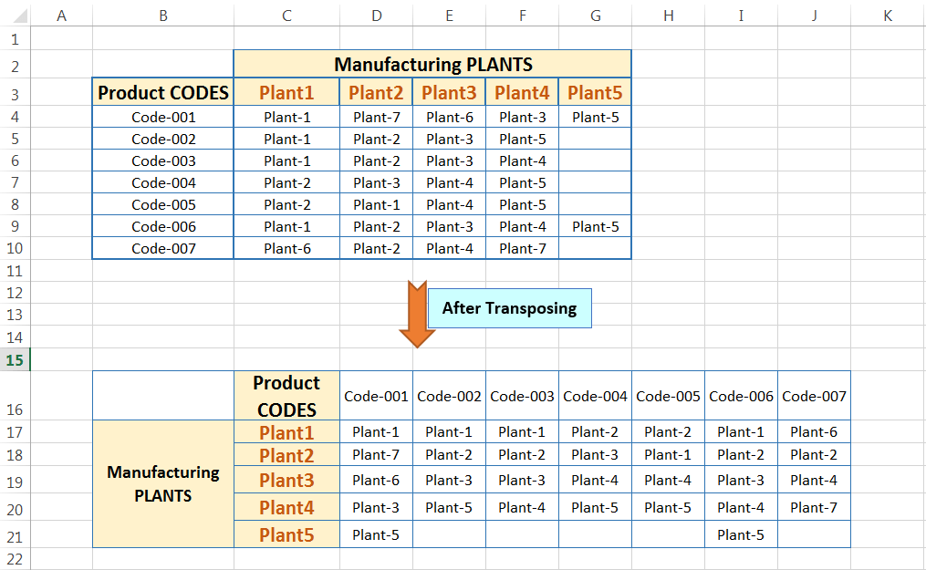
Transposing data change the orientation of a table or range of cells, which means rows become columns, and columns become rows. Any formulas in the copied range are adjusted so that they work properly when transposed.
II. HOW TO TRANSPOSE DATA IN EXCEL?
(A) METHOD 01: TRANSPOSE DATA IN EXCEL ➪ USING OF ‘TRANSPOSE’ OPTION IN THE ‘PASTE SPECIAL’ DIALOG BOX
The Transpose option in the Paste Special dialog box changes the orientation of the copied range or the data. As a result, rows become columns, and columns become rows.
Please note that we can use the ‘Transpose’ option with the other options in the ‘Paste Special’ dialog box.
Steps to Start:

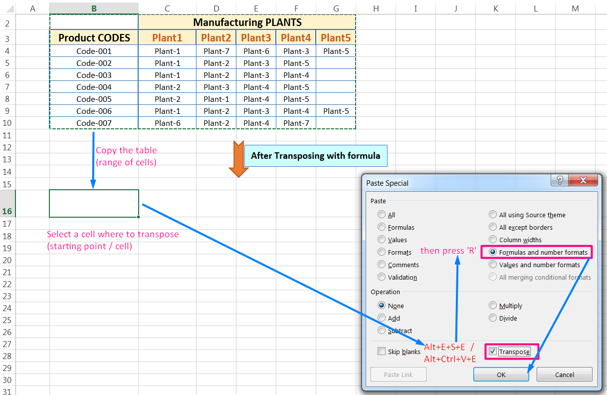
(01) Copy the table or the range of cells to be transposed (B2:G10) with Excel shortcut Ctrl+C or Choose Home ➪ Copy.
(02) Click the cell where the transposed cells to begin i.e., the cell B16.
(03) Using of Transpose Option in the ‘Paste Special’ Dialog Box:
➢ Method 1: Using excel Shortcut Alt+E+S+E or Alt+Ctrl+V+E
After selecting a cell (i.e., B16), press sequentially Alt, E, S, E; or press Alt+Ctrl+V, E which will select the ‘Transpose‘ option under the ‘Paste Special’ dialog box ➪ then click on ‘OK’ or press ‘Enter’.
As a result, Excel transposes the copied data/range into the new area where rows arrange into columns or columns into rows.
Note: After pasting the contents to their new location, press the ‘Esc‘ (Escape) key. The animated marquee is removed.
➢ Method 2: Right-click on the Mouse
After selecting a cell, just right-click on the mouse ➪ click on ‘Paste Special…’ under ‘Paste Options:’ ➪ select the checkbox of ‘Transpose’ option ➪ click ‘OK’ or press ‘Enter’.

As a result, Excel copies the selected cells in the new area, transposing rows into columns or columns into rows.
Note: After pasting the contents to their new location, press the ‘Esc‘ (Escape) key. The animated marquee is removed.
➢ Method 3: Using the Ribbon
Go to the ‘Home’ tab ➪ click the down arrow below ‘Paste’, a menu of options appears to ➪ click on ‘Paste Special…’ ➪ select the checkbox of ‘Transpose’ option ➪ click ‘OK’ or press ‘Enter’.

As a result, Excel copies the selected cells in the new area, transposing rows into columns or columns into rows.
Note: After pasting the contents to their new location, press the ‘Esc‘ (Escape) key. The animated marquee is removed.
(04) Transposing with the Formula:
While data is transposed with the Paste Special dialog box, the actual data is copied to the new area, but pastes all the formulas that reference the original data – and that is the key point. If we want to keep the formulas in transposed data, then follow the below steps:
(a) Copy the same table or the range of cells to be transposed (B2:G10) with Excel shortcut Ctrl+C or Choose Home ➪ Copy.
(b) Click the cell where the transposed cells to begin i.e., the cell B16.
(c) Then press sequentially Alt, E, S, E or press Alt+Ctrl+V, E which will select the ‘Transpose‘ option under the ‘Paste Special’ dialog box ➪ after that press ‘R‘ which will select the option ‘Formulas and number formats‘ ➪ then click on ‘OK’ or press ‘Enter’.
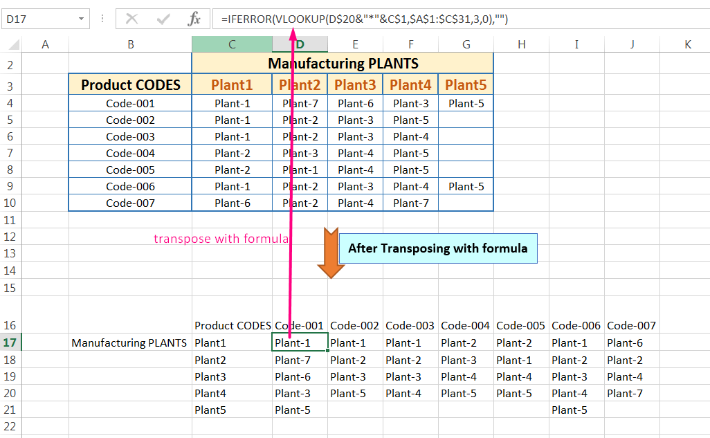
As a result, Excel transposes copied data/range with all the formulas in the new area that reference the original data.
Note: After pasting the contents to their new location, press the ‘Esc‘ (Escape) key. The animated marquee is removed.
(05) Assign the same Formatting into the Transposed data/table:
The transposed data does not necessarily take on the formatting of the original area. So we may need to format the area.
In this case, we assign the cell formatting on the same transposed data.
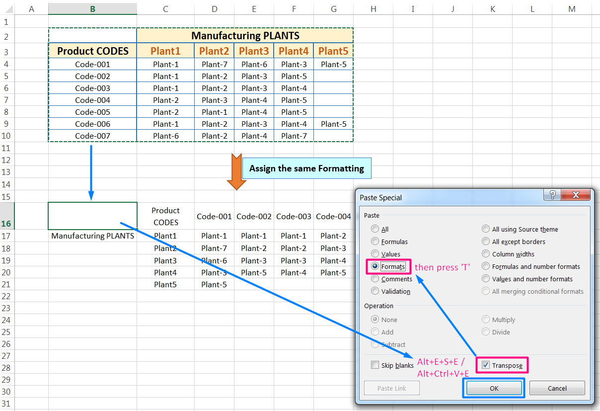
(a) Copy the original table or the range of cells once again, i.e., B2:G10 either with Excel shortcut Ctrl+C or using the ribbon Home ➪ Copy.
(b) Click the first cell of the transposed data or the range, i.e., the cell B16.
(c) Then press sequentially Alt, E, S, E or press Alt+Ctrl+V, E which will select the ‘Transpose‘ option under the ‘Paste Special’ dialog box ➪ just after press ‘T‘ which will select the option ‘Formats‘ ➪ then click on ‘OK’ or press ‘Enter’.
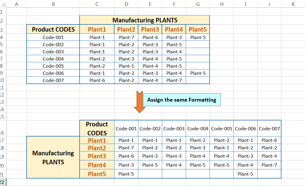
As a result, Excel assigns the same formatting of the original data/table into the transposed data or table.
Note: After pasting the contents to their new location, press the ‘Esc‘ (Escape) key. The animated marquee is removed.
➢ Conclusion
01. The Transpose option in the Paste Special dialog box pastes all the formulas.
02. To assign the formulas into the transposed data/table, we need to use both options like the ‘Transpose’ option and the ‘Formulas and number formats’ options respectively in the ‘Paste Special’ dialog box.
03. If we want to assign the formatting on the same transposed data/table, again we use both options like the ‘Transpose’ option and the ‘Formats’ option respectively.
(B) METHOD 02: TRANSPOSE DATA IN EXCEL ➪ USING EXCEL ‘TRANSPOSE’ FUNCTION
The Excel TRANSPOSE function is an array function, which essentially converts the horizontal array to a vertical array and vice versa. In other words, the TRANSPOSE() function can change the structure of a table or a range, inverting the data so that all the rows become columns, and all the columns become rows.
➢ The Syntax for the TRANSPOSE Function:
The only argument for the Excel TRANSPOSE() function is the array argument, which identifies the range of the original dataset.
➢ The Differences Between the Excel TRANSPOSE Function & Transpose Paste Option:
Using the TRANSPOSE() function in Excel is similar to using the Transpose paste option, but there are several important differences.
(i) The TRANSPOSE() function creates a linked table that’s bound to the original data, which means that if we change the original table, the transposed table also changes. The Transpose paste option does not do it.
(ii) The other key point is that the Excel TRANSPOSE() function only works as an array function, So, we must enter it into the entire destination range simultaneously, and must press Ctrl+Shift+Enter to apply the function. Keep in mind the destination range must contain the same number of rows as the original dataset has columns, and it must have the same number of columns as the original dataset has rows.
(iii) If we selected one of the cells in the transposed range to display the array function, more clearly a single function that exists in each cell in the range.
(iv) The TRANSPOSE() function in Excel does not carry formatting to the transposed range; we must reformat the new dataset if we want the formatting to match.
➢ Steps to Start
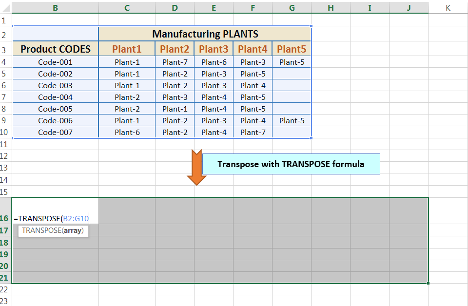
(01) Select the range of cells to be transposed (i.e., B2:G10).
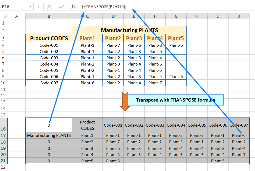
Make a note of its size in rows and columns (means the number of columns and rows it contains). Range B2:G10 has 9 rows and 6 columns which will be transposed to the target range B16:J21 which has 6 rows and 9 columns.
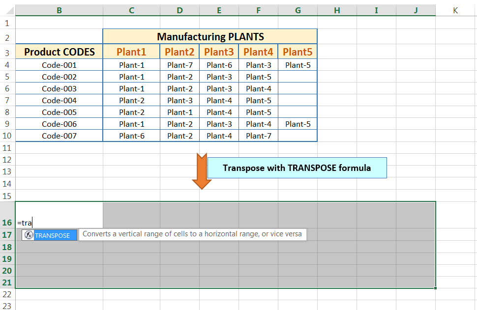
(02) Select the appropriately sized area (grid of cells) where we want to insert the transposed cells.
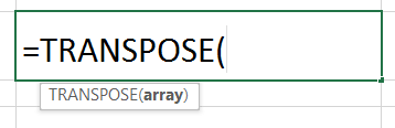
(03) Press the equal sign (=) in cell B16 and enter the TRANSPOSE() formula.
The TRANSPOSE() formula requires one argument, which is the range of cells you want to transpose. Here’s an example: =TRANSPOSE(B2:G10). Don’t press Enter yet.
(04) Commit the function by pressing Ctrl+Shift+Enter, in that order of keystrokes.
This step inserts the formula into all the selected cells as an array formula.
Interestingly, the formula in the target range will be the same for all cells in the range: {=TRANSPOSE(B2:G10)}
The curly brackets ({}) surrounding the formula designate the range as an array. The only way to create an array is to use the Ctrl+Shift-Enter sequence of keystrokes (the brackets are automatically produced).
Note that physically typing the brackets will not create an array in the range.
Note: After pasting the contents to their new location, press the ‘Esc‘ (Escape) key. The animated marquee is removed.
[Tip: Editing array formulas can be a challenge. To remove or replace an array formula, we need to first select all the cells that use it. If we have a large array formula, then the helpful trick is to use the ‘Go To‘ command to select the array formula cells.
First, select one of the cells that has the array formula ➪ Press Ctrl+G to show the ‘Go To’ dialog box ➪ Next, click the Special button or press Alt+S ➪ choose “Current array” ➪ then click ‘OK‘ or press ‘Enter’. Excel selects the entire group of cells that uses this array formula]
(C) METHOD 03: TRANSPOSE DATA IN EXCEL ➪ USING COMBINED FUNCTIONS OF COUNTIFS(), PIVOT TABLE, VLOOKUP(), INDIRECT(), & IFERROR()
We cannot easily transpose a data where one column continues vertically (column-wise) whereas the other column needs to arrange horizontally (row-wise). So, in that case, neither TRANSPOSE () formula nor ‘Transpose’ option in the Paste Special dialog works out.
Here, we use combined functions such as COUNTIFS, PivotTable, VLOOKUP, INDIRECT, and IFERROR step by step to transpose data (columns to rows) in Excel.
➢ Steps to Start
In the following example, there is a list of cells A2:B31, where Column A grips ‘Product Codes’, whereas column B ‘Manufacturing Plants’. Here we like to arrange the ‘Manufacturing Plants’ horizontally (row-wise) against the ‘Product Code’.

➢ Step 1: Find out Duplicate Value with the COUNTIFS Function
(01) In the first step, we find out the duplicate count of Product Codes. Thus we apply the COUNTIFS function (or COUNTIF function). Preferably we apply the COUNTIFS function in column C.
Place an equality sign (=) in cell C2 and type ‘coun…’, select COUNTIFS from the below suggestion list of Down Arrow key (⬇), and press the ‘Tab’ key. COUNTIFS syntax appears with an open parenthesis.

Note: the upper or lower case does not matter in syntax, Excel by default considers it in upper case.
(02) Select the cell A2 as criteria_range1, the first argument of the COUNTIFS function.

Then press full stop (.), Excel considers that the range starts from the same cell (or the same point) and it seems to be A2:A2.
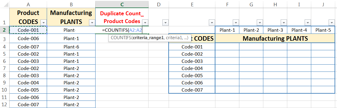
Place a comma (,) to move to the next argument.
(03) Again select the cell A2 as criteria1, the second argument of the COUNTIFS function.

(04) Using of Cell References:
Just select the first part (left part of the range) of the criteria_range1 and fix it by pressing the F4 Key once which will convert the cell from the relative cell reference to the absolute cell reference.
Thus, the criteria_range1 seems to be $A$2:A2.

(05)Finally, press ‘Enter‘ to apply the formula in cell C2 and get the value as a result.
(06) Extending the formula Down to the Range: Alt+E+S+R / Alt+Ctrl+V+R
After getting the result, copy the cell C2 with Excel shortcut Ctrl+C ➪ making a selection down to the range with the Shift + Down arrow (⬇) ➪ press sequentially Alt+E+S+R (such as Alt, E, S, R) / Alt+Ctrl+V+R (such as Alt+Ctrl+V, R) which will select the option ‘Formulas and number formats‘ in the ‘Paste Special’ dialog box ➪ Click on ‘OK’ or press ‘Enter’ to accept the formula.

• Alternatively, Copy (Ctrl+C) the cell C2 ➪ making a selection down to the range with Shift + Down arrow (⬇) ➪ paste (Ctrl+V or simply press ‘Enter’) down to the range.
(Remember that the same cell formatting copied in each cell).
• Alternatively, select the cell that has the formula we want to fill down to the range ➪ either double click on the fill handle or drag the fill handle down to the range.
(Remember that the same cell formatting also copied in each cell).
➢ Step 2: Creating a PivotTable of a Dataset
• Method 1: Using Excel Shortcut Alt+D+P
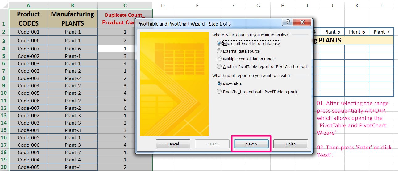
(01) Click anywhere in the dataset ➪ it is the best way to select the entire dataset by pressing Ctrl+A before creating a PivotTable.
(02) Then press sequentially Alt+D+P (likes Alt, D, P) opens the ‘PivotTable and PivotChart Wizard’, the Step1 of 3.
(03) Press ‘Enter’ or click ‘Next’ to move to Step 2 of 3, already range is selected in ‘Range:’ box.
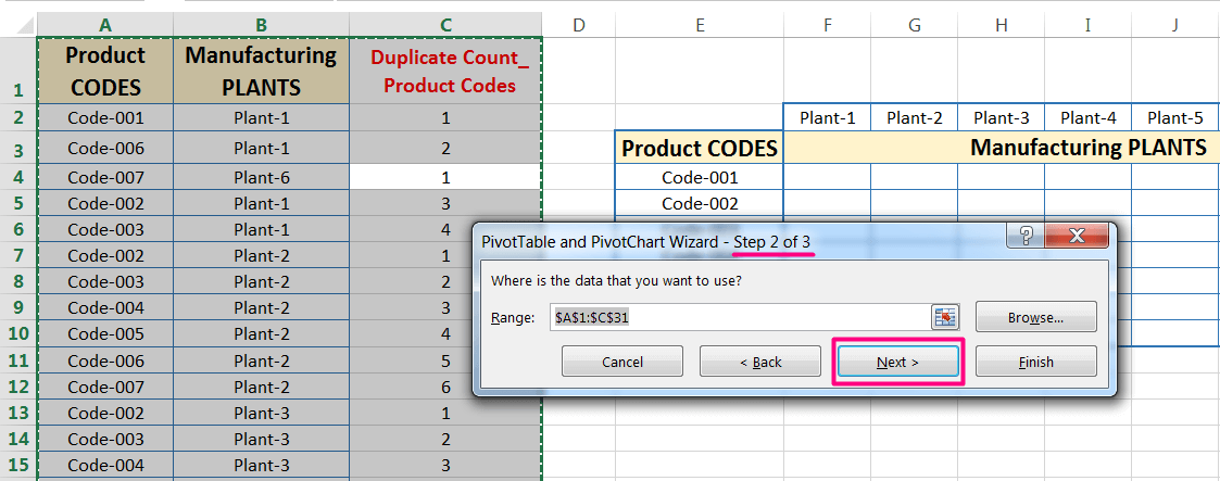
(04) Again press ‘Enter’ or click ‘Next’ to move to Step 3 of 3, indicates the location for the pivot table. The default location is on a new worksheet, but we can specify any range on any worksheet, including the existing worksheet that contains the data.
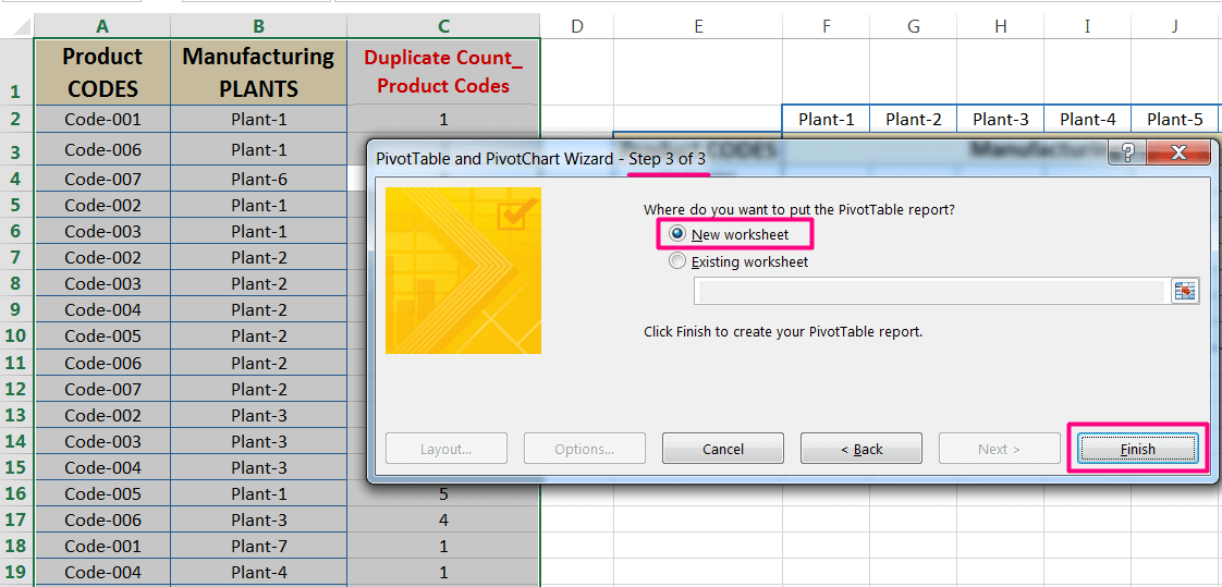
Finally, press ‘Enter’ or click ‘Finish’, and Excel creates an empty pivot table and displays its PivotTable Field List task pane.
• Method 2: Using Excel Shortcut Alt+N+V
(01) Click anywhere in the dataset ➪ press Ctrl+A selecting the entire dataset before creating a PivotTable.
(02) Then press sequentially Alt+N+V (Alt, N, V) opes the ‘Create PivotTable’ dialog box, where the range is already selected in the ‘Table/Range:’ box and the bottom section of the dialog box indicates the location for the pivot table.
The default location is on a new worksheet, if not please select the ‘New Worksheet‘ checkbox. However, we can specify any range on any worksheet, including the existing worksheet that contains the data.
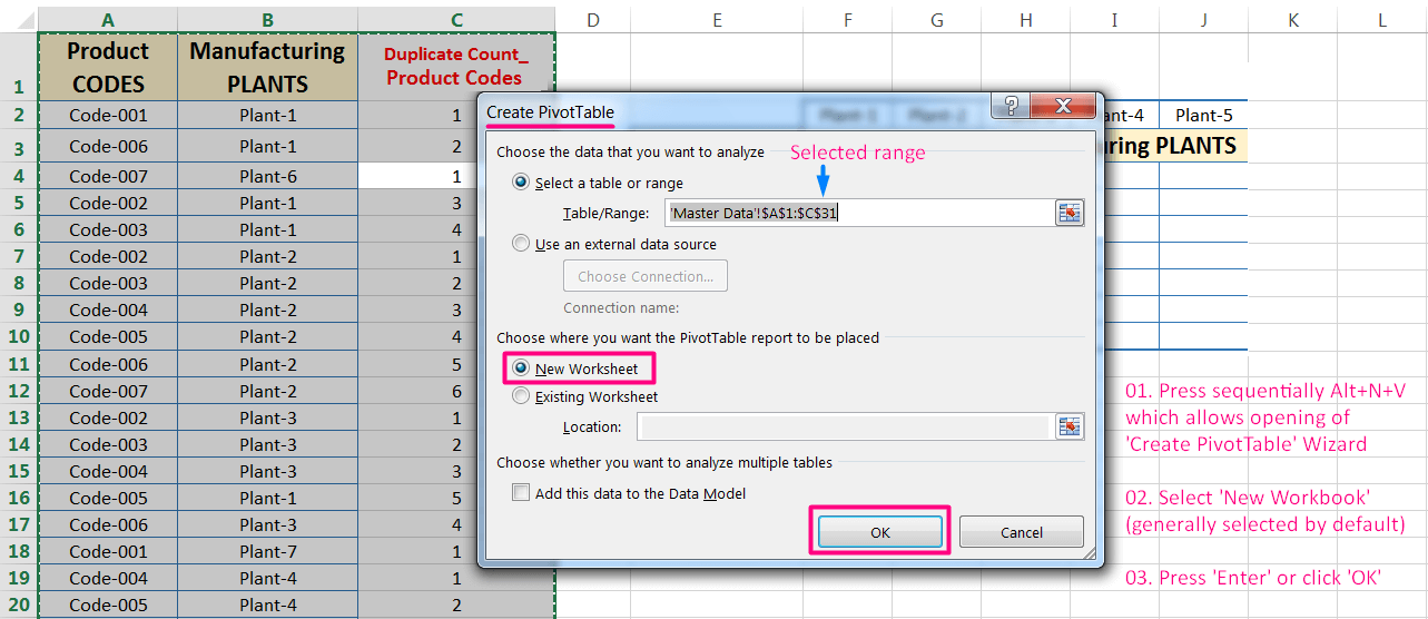
Finally, press ‘Enter’ or click ‘OK’, and Excel creates an empty pivot table and displays its PivotTable Field List task pane.
• Method 3: Using the Ribbon
(01) Click anywhere in the dataset ➪ press Ctrl+A selecting the entire dataset before creating a PivotTable.
(02) Go the ‘Insert’ tab ➪ click on the ‘Pivot Table’ button, which displays the ‘Create PivotTable’ dialog box where the range is already selected in the ‘Table/Range:’ box and in the bottom section by default selected ‘New Worksheet’, if not please select the ‘New Worksheet‘ checkbox.
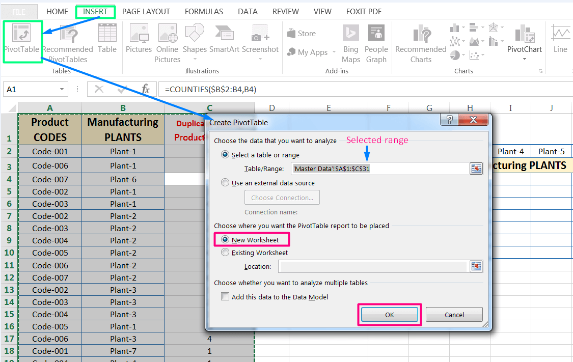
Finally, press ‘Enter’ or click ‘OK’, and Excel creates an empty pivot table and displays its PivotTable Field List task pane.
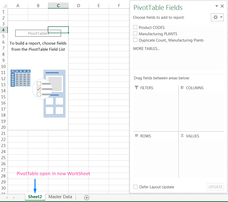
➢ Step 3: Laying out the PivotTable
Next, set up the actual layout of the pivot table. We can do so by using either of any methods:
• Method 1: Drag the field names (at the top of the PivotTable Fields task pane) to one of the four areas at the bottom of the PivotTable Field task pane.
• Method 2: Place a checkmark next to the item. Excel places the field into one of the four areas at the bottom.
• Method 3: Right-click a field name at the top of the PivotTable Fields task pane and choose its location from the shortcut menu.

Now drag the items from the top of the PivotTable Field task pane to the areas in the bottom of the PivotTable Field task pane.
01. Drag the ‘Product CODES’ field in the ‘Rows’ area.
02. Drag the ‘Manufacturing PLANTS’ field in the ‘Rows’ area just below the ‘Product CODES’.
03. Drag the ‘Duplicate Count_ Manufacturing Plants’ field in the ‘FILTERS’ area.
The pivot table shows the ‘Manufacturing PLANTS’ for each ‘Product CODES’ type, The pivot table updates itself automatically after making any changes in the PivotTable Fields task pane.
➢ Step 4: Changing Layout to Classic PivotTable Layout
In this step, we change the layout to the Classic Pivot Table layout. We can do it in 2 ways:
• Method 1: Using Right-Click anywhere in the Pivot Table
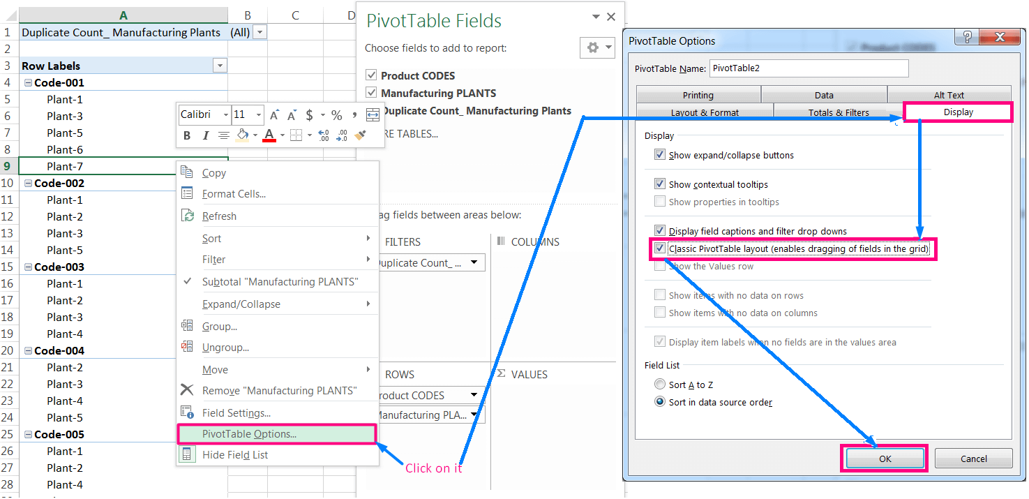
Right-click somewhere on the pivot table ➪ select ‘PivotTable Options…’, which displays the ‘PivotTable Options’ dialog box ➪ select the checkbox ‘Classic PivotTable layout…’ under ‘Display’ tab ➪ click ‘OK’ to accept the layout.
• Method 2: Using the Ribbon
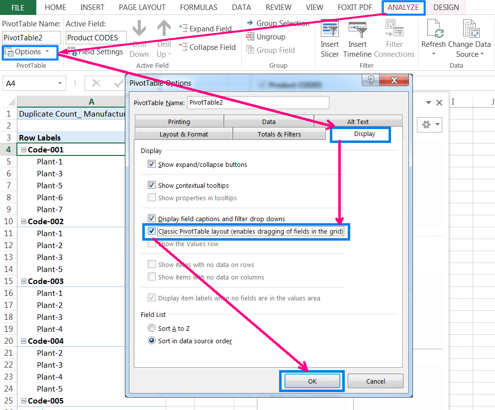
Select a cell somewhere in the pivot table ➪ then go to the ‘ANALYZE’ tab of the PivotTable Tools (showing on the ribbon) ➪ click ‘Options’ drop-down in the PivotTable section, which displays the ‘PivotTable Options’ dialog box ➪ select the checkbox ‘Classic PivotTable layout…’ under ‘Display’ tab ➪ click ‘OK’ to accept the layout.
➢ Step 5: Removing Subtotals
Subtotals are an essential feature of pivot table reporting, however, sometimes it creates obscure to visualize, and sometimes there is no need to show subtotals.
We can suppress subtotals in 2 ways:
• Method 1: Using Right-Click on any of the Subtotal Cells in the Pivot Table
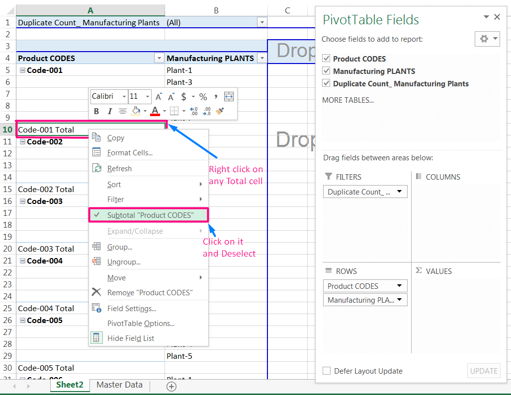
Right-click on any of the Subtotal cells ➪ Click on Subtotal “Product CODES”, which removes subtotals for the Product Codes.
• Method 2: Using the Ribbon
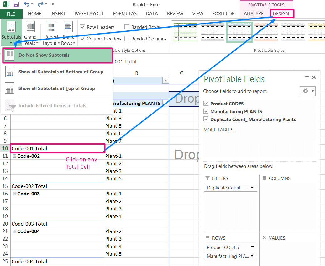
Select a subtotal cell ➪ then click the ‘DESIGN’ tab of the PivotTable Tools (showing on the ribbon) ➪ click the ‘Subtotals’ drop-down ➪ choose ‘Do Not Show Subtotals’, which allows turning off subtotals for the Product Codes.
➢ Step 6: Select Multiple Items from the Table Filter
Table Filter is a field that has a page orientation in the pivot table, through which we can display only one item (or all items) in a page field at one time. In the previous version of Excel, a table filter was known as a Page field.
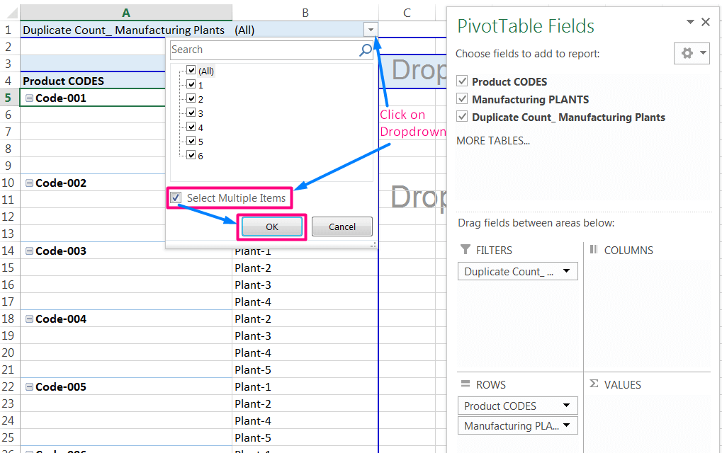
Click on the drop-down of Table Filter ➪ activate the checkbox by clicking on ‘Select Multiple Items’, as a result, all the checkboxes are checked by default ➪ click ‘OK’.
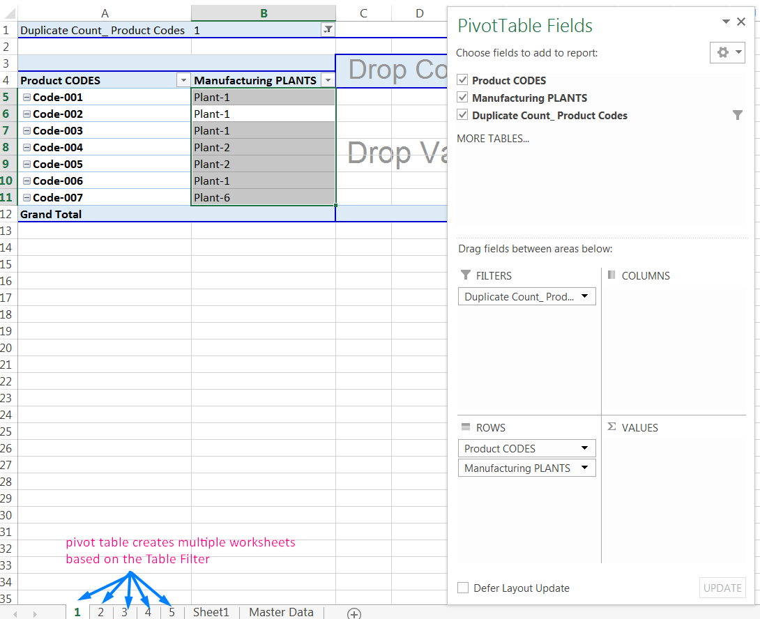
➢ Step 7: Creating Multiple Worksheets Based on the Table Filter
Based on the Table Filter, we can create multiple worksheets in the following ways:

Click on the Table Filter area ➪ go to the ‘ANALYZE’ tab in the PivotTable Tools (showing on the ribbon) ➪ click the ‘Options’ drop-down in the PivotTable section ➪ click ‘Show Report Filter Pages…’, the second item of a drop-down list ➪ displays ‘Show Report Filter Pages’ dialog box ➪ click ‘OK’.
As a result, multiple worksheets have been created based on Table Filter.
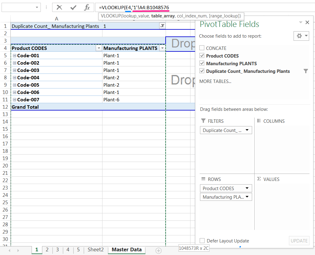
➢ Step 8: Assign the VLOOKUP formula with a Single Worksheet
(01). Place an equality sign (=) in cell F4 and type ‘vlo…’, select VLOOKUP from the below suggestion list of Down Arrow key (⬇), and press the ‘Tab’ key. VLOOKUP syntax appears with an open parenthesis.
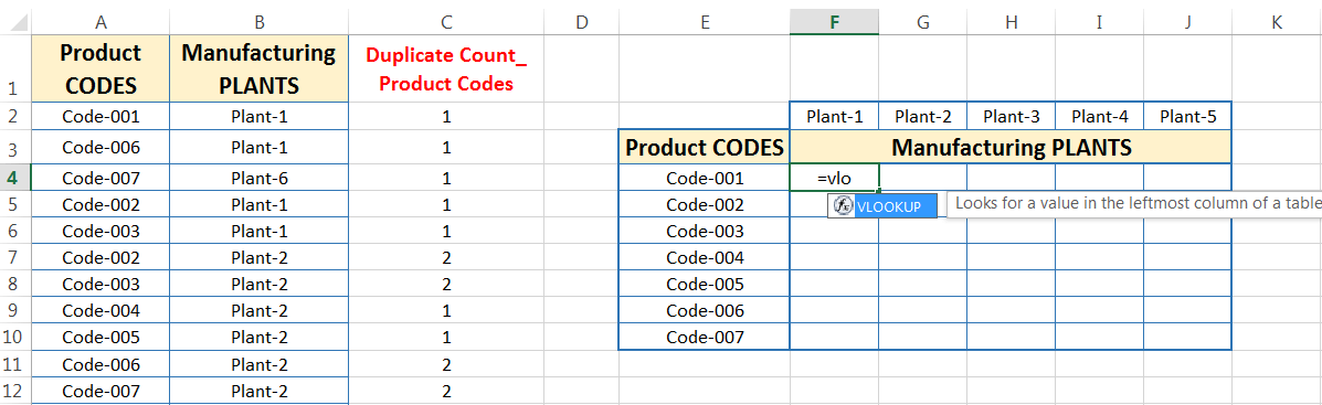
Note: The upper or lower case does not matter for the syntax, Excel by default considers it in upper case.
(02). Then, select cell E4 as lookup_value, the first argument of VLOOKUP. Cell E4 refers to one of the Product Codes.
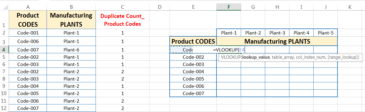
Place a comma (,) to move to the next argument.
(03). Go to any worksheet, for example, here we move to ‘1’ worksheet. Select the entire range (A4:B1048576) as a table_array with Ctrl+Shift+Right Arrow (➡) and Ctrl+Shift+Down Arrow (⬇).
Cell A4 is the first cell of the lookup column, whereas cell B1048576 is the end cell of the range.
Keep in mind that we should extend the range downward (or vertically, or column-wise) till the end of the worksheet. Because different worksheets have different ranges, so we try to select the highest range downward to avoid an error.
(04). Put a value 2 as a column_index_number, the third argument of VLOOKUP. Column number 2 refers to EXCEL to move 2 columns at the right starting from the lookup column. It indicates ‘Manufacturing Plants’.

For example, the lookup column in our database is Column A and VLOOKUP retrieves data from Column B, just 2 columns right considering column A.
Place a comma (,) to move to the next argument.
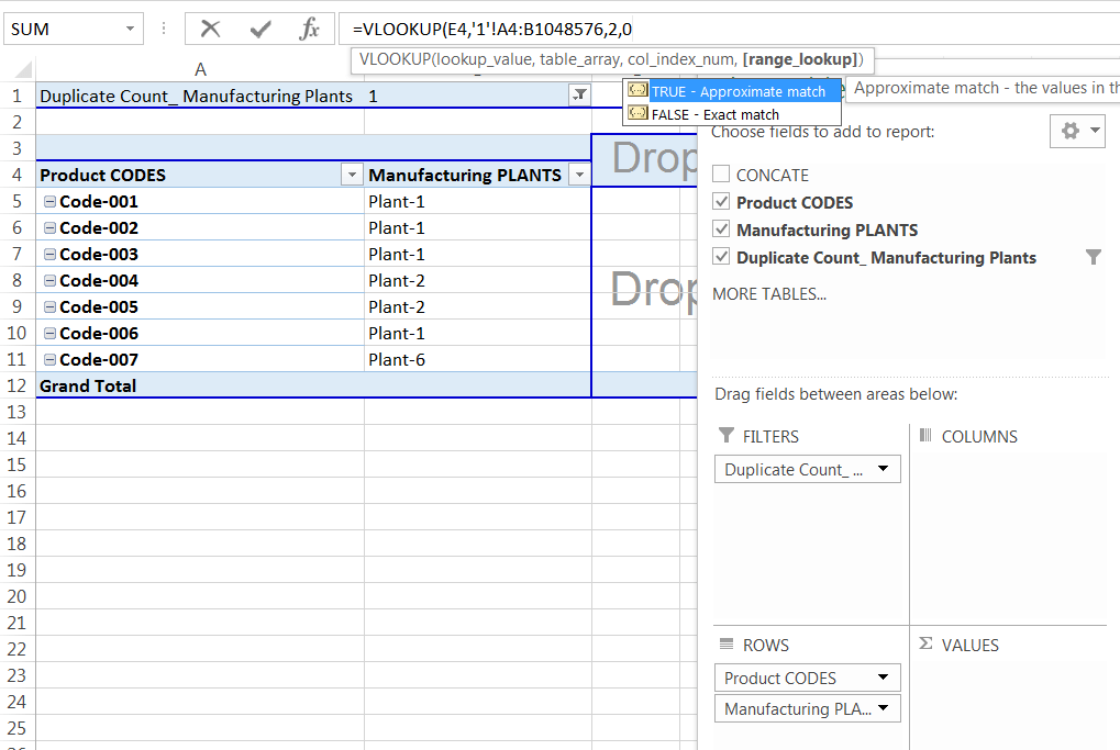
(05). As we find an exact match, so put 0 (zero) or False in place of range_lookup, the fourth argument of VLOOKUP.
(06). Press ‘Enter‘ to accept the formula. Excel by default closes the last parenthesis.
=VLOOKUP(E4,‘1‘!A4:B1048576,2,0)
➢ Step 9: Mentioned Worksheet Name above the Table/Range
We should mention the number of duplicate counts serially till the maximum number.
For example, there is a maximum count of duplicate value is 5, and based on that 5 new worksheets have been created, and we should mention their names above the table/range horizontally.

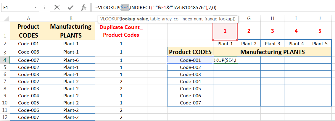
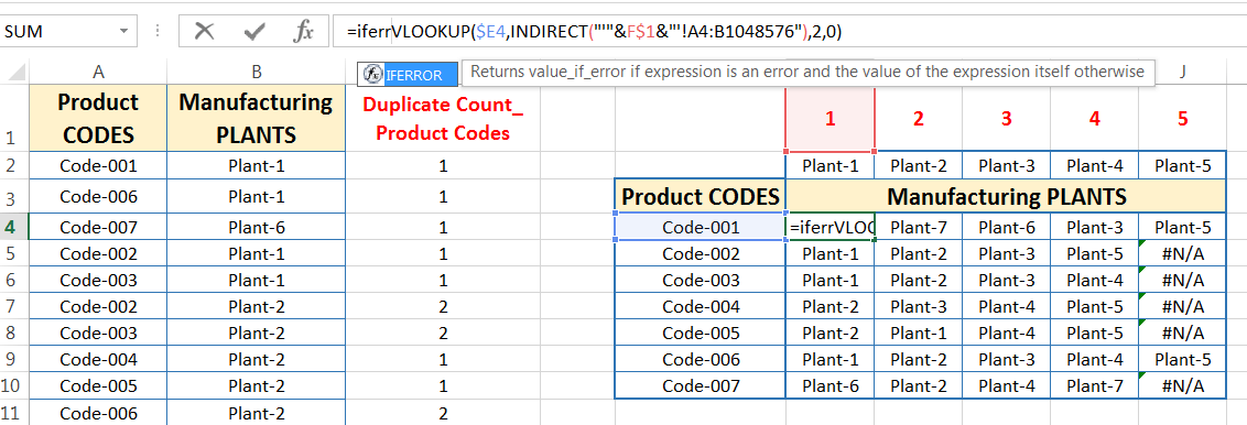
➢ Step 10: Using of INDIRECT function in the VLOOKUP Formula
This step is very important. Now we assign the INDIRECT function within the VLOOKUP formula that helps in retrieving data from multiple worksheets (or in short form Sheets).
• The Syntax for the INDIRECT function:

We use the INDIRECT function in the position of lookup_array. Follow the mentioned figure below.

• Steps to Start:
01. Just type ‘ind…’ starting of the table_array and select the INDIRECT function from the below suggestion list of Down Arrow key (⬇), and press the ‘Tab’ key. The syntax of the INDIRECT function appears with an open parenthesis.

Wrap the single quotation mark with the double quotation mark likes “‘“.
02. Then place an ampersand symbol (&).
03. Replace the sheet name with the cell reference which refers to a specific sheet name. For example, sheet name ‘1’ replaces with the cell reference ‘F1’, where F1 refers to sheet ‘1’. Using cell references within the INDIRECT function makes the VLOOKUP formula dynamic, which means the VLOOKUP formula is able to retrieve data from multiple sheets.
04. Again place an ampersand symbol (&) after the cell reference.
05. The rest part of the lookup_array must be quoted with a double quotation mark, such as “‘!A4:B1048576“.
06. Then close the parenthesis of the INDIRECT Function. Thus, it will be considered as a ref_text of the INDIRECT function.

➢ Step 11: Using Cell References
01. This is an important section. At first, select the lookup_value and press the F4 key three times to convert from the relative cell reference to the mixed cell reference (where the absolute column but the relative row).
Thus, the lookup_value seems to be $E4.
02. Then select the cell reference F1 inside the INDIRECT function and press the F4 key twice to convert it from the relative cell reference to the mixed cell reference (where the row becomes absolute but the column remains relative).
Thus, it seems like F$1.

Press ‘Enter’ to accept the changes in the formula.
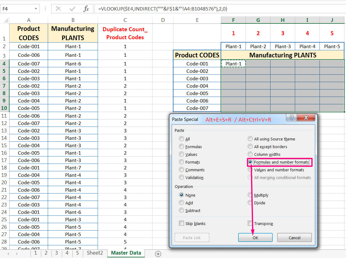
➢ Step 12: Extending the Formula into the Entire Ranges: Alt+E+S+R / Alt+Ctrl+V+R
After getting the result, copy the cell F4 with Excel shortcut Ctrl+C ➪ making a selection of the entire ranges with Shift+ Right arrow (➡), Down arrow (⬇ ) ➪ press sequentially Alt+E+S+R (such as Alt, E, S, R) / Alt+Ctrl+V+R (such as Alt+Ctrl+V, R) which will select the option ‘Formulas and number formats‘ under the ‘Paste Special’ dialog box ➪ click on ‘OK’ or press ‘Enter’ to accept the formula.
Note: After pasting the contents to their new location, press the ‘Esc‘ (Escape) key. The animated marquee is removed.
➢ Step 13: Replacing Errors with the IFERROR function
An error value is returned when a formula does not contain sufficient or valid arguments to return a value. The error values always preventing Excel from returning a calculated value. An error value begins with a number sign (#) followed by an error name that indicates the type of error. Most common error values are # N/A, #DIV/0, #NAME, #NUM, #REF, #VALUE.
The IFERROR function is a logical function which returns a value if a formula evaluates to an error; otherwise, it returns the result of the formula.
The syntax for the IFERROR function is

• value is a cell reference or formula.
• value_if_error is the message to be displayed if the value argument returns an error. We replace these errors with a character (such as space “ ” or zero 0 or any text within a double quotation mark, for example, “No value”) a snap. If Excel does not detect an error, the value is displayed as a result.
• Steps to Start:
Edit the VLOOKUP formula in cell F4, we place the IFERROR function at the starting of the VLOOKUP formula. After the VLOOKUP formula place a comma (,). As a result, the entire VLOOKUP formula considers a value argument. After the placing comma, move to the next argument value_if_error where we use space (“ ”) as a character.
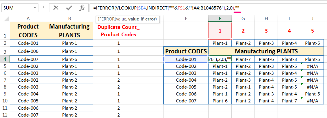
As a result, if the VLOOKUP function returns the error value #N/A, the second argument in the IFERROR function is executed, and space (“ ”) is displayed.
Press ‘Enter’ before the closing of parenthesis and Excel returns a warning message “We found a typo in your formula and tried to correct it to:”, either we press ‘Enter’ or click ‘Yes’ to accept this correction. EXCEL by default closes the last parenthesis and returns the result.
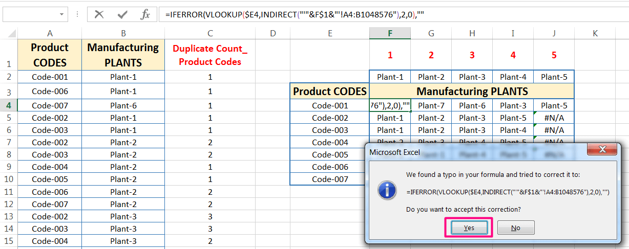
Then the formula seems to be:
=IFERROR(VLOOKUP($E4, INDIRECT(“‘“&F$1&”‘!A4:B1048576″), 2, 0),” “)
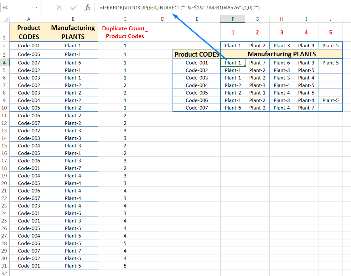
➢ Step 14: Again Extending the Formula into the Entire Ranges: Alt+E+S+R / Alt+Ctrl+V+R
This step is similar to Step 12.

After getting the result, copy the cell F4 with Excel shortcut Ctrl+C ➪ making a selection of the entire ranges with Shift+ Right arrow (➡), Down arrow (⬇) ➪ press sequentially Alt+E+S+R (such as Alt, E, S, R) / Alt+Ctrl+V+R (such as Alt+Ctrl+V, R) which will select the option ‘Formulas and number formats‘ under the ‘Paste Special’ dialog box ➪ click on ‘OK’ or press ‘Enter’ to accept the formula.
Note: Excel displays an animated marquee around cells that have been cut or copied. After pasting the contents to their new location cancel the animated marquee by pressing the ‘Esc‘ (Escape) key.
(D) METHOD 04. TRANSPOSE DATA IN EXCEL ➪ USING COMBINED FUNCTIONS OF COUNTIFS(), CONCATENATE(), VLOOKUP(), & IFERROR()
There is an alternate method for transpose columns to rows in Excel with the help of COUNTIFS, CONCATENATE, VLOOKUP, and IFERROR functions.
However, we use a combined process with them step by step for transposing data (columns tox rows) in Excel.
➢ Steps to Start
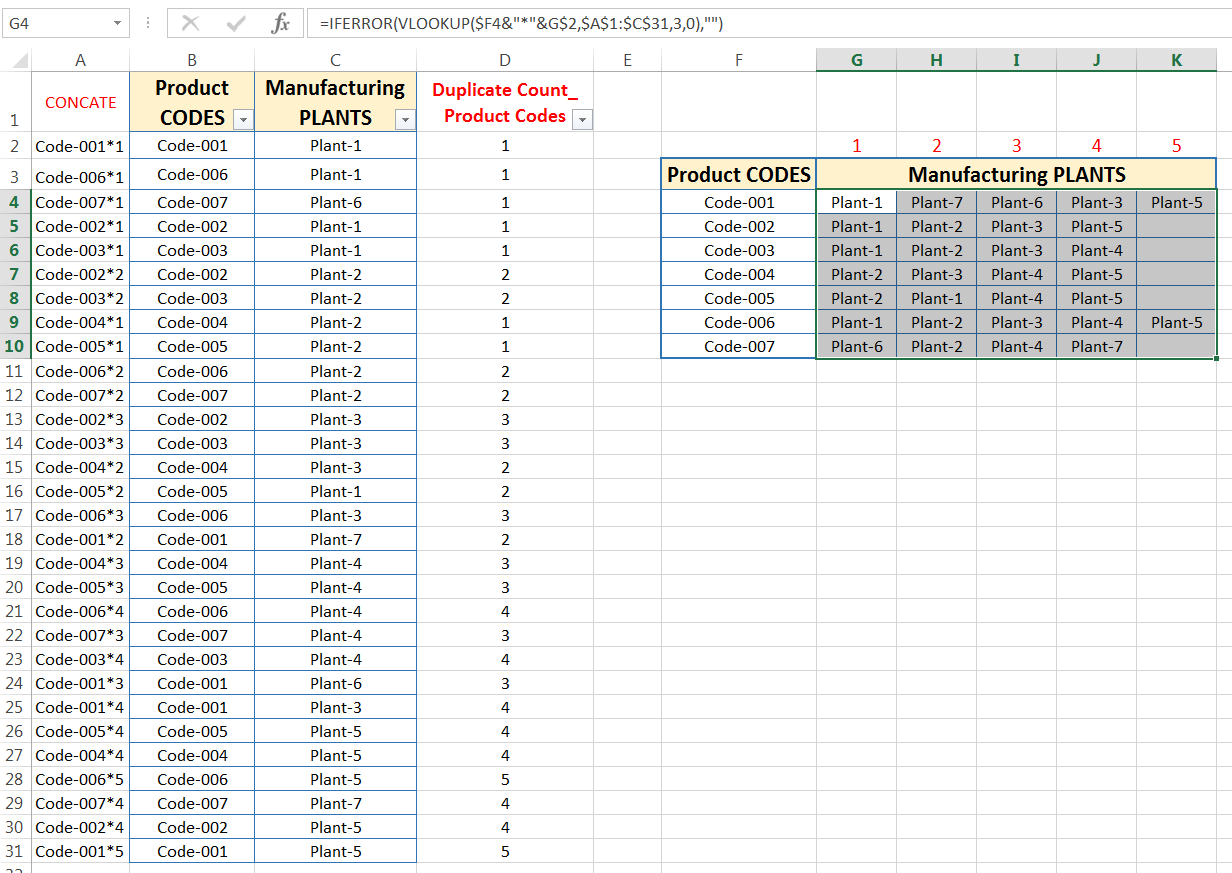
In the following example, there is a list of cells A2:B31, where Column A grips ‘Product Codes’, whereas column B ‘Manufacturing Plants’. Here we like to arrange the ‘Manufacturing Plants’ horizontally (row-wise) against the ‘Product Code’.
• Step 1: Find out Duplicate Value with the COUNTIFS Function
In the first step, we find out the duplicate count of Product Codes with the COUNTIFS function (or COUNTIF function) in column C (especially apply in cell C2).
(i). Place an equality sign (=) in cell C2 and type ‘coun…’, select COUNTIFS from the below suggestion list of Down Arrow key (⬇), and press the ‘Tab’ key. COUNTIFS syntax appears with an open parenthesis.
(ii). Select the cell A2 as criteria_range1, the first argument of the COUNTIFS function.
Then press full stop (.), Excel considers that the range starts from the same cell (or the same point) and it seems to be A2:A2.
Place a comma (,) to move to the next argument.
(iii) Again select the cell A2 as criteria1, the second argument of the COUNTIFS function.
(iv) Using Cell References:
Just select the first part (left part of the range) of the criteria_range1 and fix it by pressing the F4 Key once which will convert the cell from the relative cell reference to the absolute cell reference.
Thus, the criteria_range1 seems to be $A$2:A2.
=COUNTIFS($A$2:A2,A2)

• Step 2: Extending the Formula Downward (Vertically): Alt+E+S+R / Alt+Ctrl+V+R
After getting the result, copy the cell C2 with Excel shortcut Ctrl+C ➪ making a selection downward (vertically) with Shift + Right arrow (➡), Down arrow (⬇ ) ➪ press sequentially Alt+E+S+R (such as Alt, E, S, R) / Alt+Ctrl+V+R (such as Alt+Ctrl+V, R) which will select the option ‘Formulas and number formats‘ under the ‘Paste Special’ dialog box ➪ click on ‘OK’ or press ‘Enter’ to accept the formula.

Note: After pasting the contents to their new location, press the ‘Esc‘ (Escape) key. The animated marquee is removed.
• Step 3: Insert a Column at the beginning of a Dataset and Name it
Select column A with Ctrl+Spacebar or click on column A ➪ then press the Ctrl + Plus (+), a new column has been inserted. As a result, the ‘Product CODES’ column by default has been shifted to the right side (i.e., shifted to column B).
=COUNTIFS($B$2:B2,B2)
Named the column as a ‘CONCATE‘.

• Step 4: Using the CONCATENATE() Function
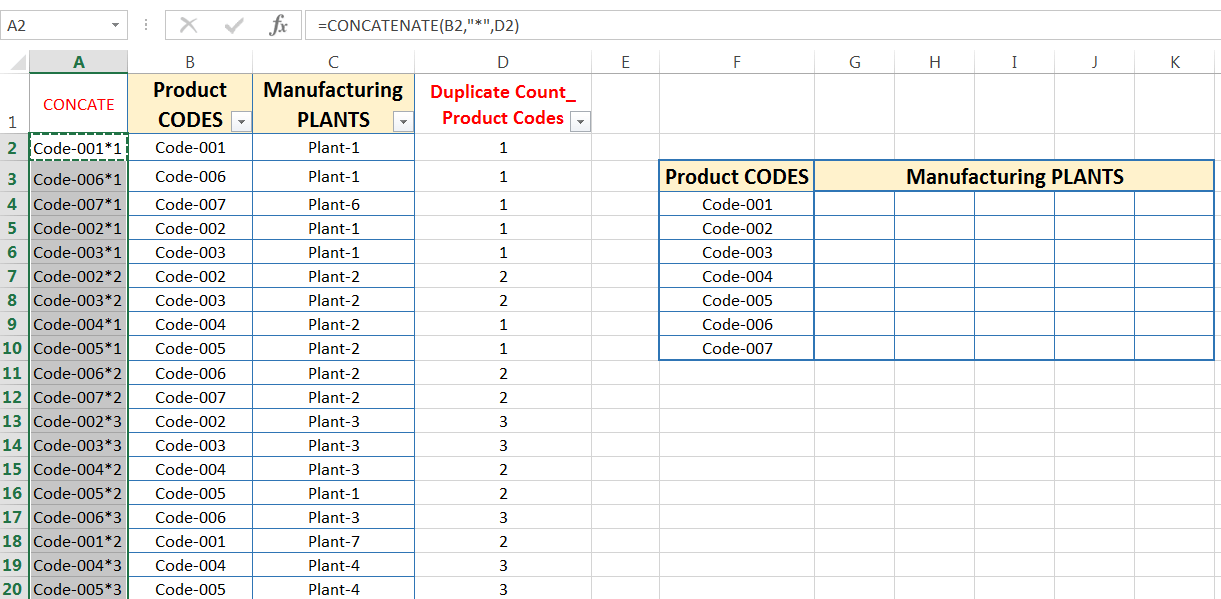
We apply the CONCATENATE function in cell A2.
In the CONCATENATE function, join the cell B2 and D2 with an asterisk (*) separator, where cell B2 refers to ‘Product CODE‘, and cell D2 refers to ‘Manufacturing PLANT‘. A separator (like an asterisk “*“) is used between them. Instead of it, we can use underscore “_”, dash “-“, divide “/”, etc., as a separator.
=CONCATENATE(B2,”*“,D2)

• Step 5: Extending the Formula Downward (Vertically): Alt+E+S+R / Alt+Ctrl+V+R
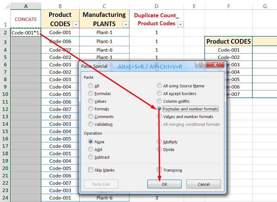
After getting the result, copy the cell A2 with Excel shortcut Ctrl+C ➪ making a selection downward (vertically) with Shift + Right arrow (➡), Down arrow (⬇ ) ➪ press sequentially Alt+E+S+R (such as Alt, E, S, R) / Alt+Ctrl+V+R (such as Alt+Ctrl+V, R) which will select the option ‘Formulas and number formats‘ under the ‘Paste Special’ dialog box ➪ click on ‘OK’ or press ‘Enter’ to accept the formula.
Note: Press the ‘Esc‘ (Escape) key. The animated marquee is removed.
• Step 6: Mentioned Worksheet Name above the Table/Range
We should mention the number of duplicate counts serially till the maximum number.
For example, there is a maximum count of duplicate value is 5, and based on that 5 new worksheets have been created and we should mention their names above the table/range horizontally.

• Step 7: Assign the VLOOKUP formula with Multiple Criteria
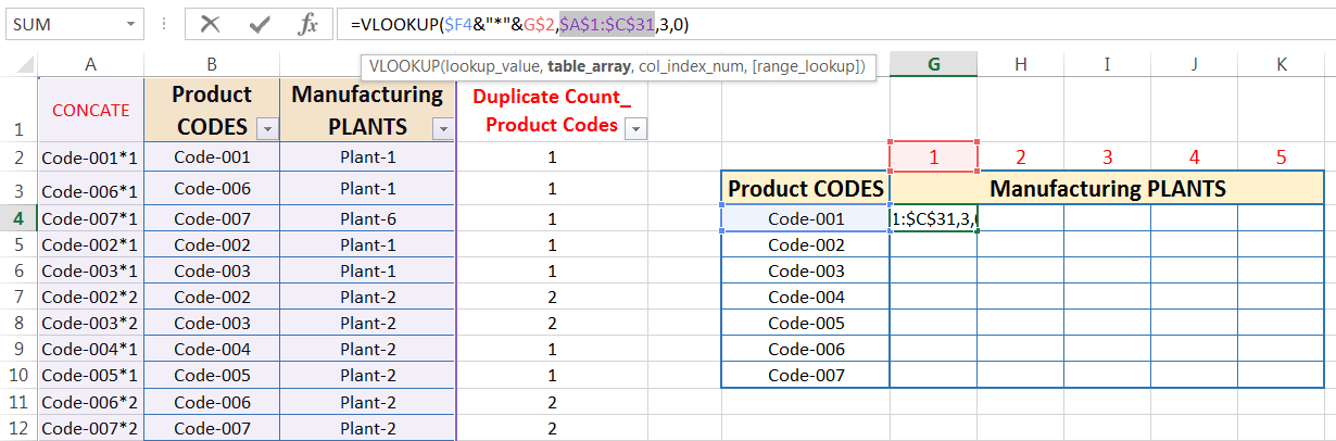
(i). Place an equality sign (=) in cell G4 and type ‘vlo…’, select VLOOKUP from the below suggestion list of Down Arrow key (⬇), and press the ‘Tab’ key. VLOOKUP syntax appears with an open parenthesis.
Note: The upper or lower case does not matter for the syntax, Excel by default considers it in upper case.
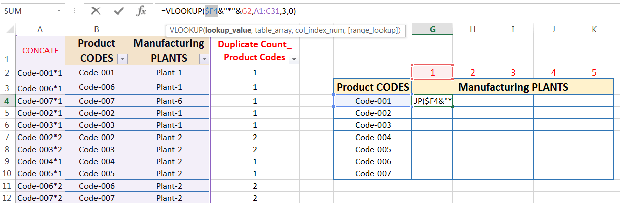
(ii). First, select a cell F4 then use an ampersand (&) symbol to concatenate the cell G2 and use an asterisk (*) symbol as a separator between them. We should place the separator in a double-quoted.
Cell F4 refers to Product CODE whereas cell G2 refers to the numeric value 1 (the lowest value of the duplicate count).
=VLOOKUP(F4&“*“&G2
The concatenated multiple criteria make the lookup_value, the first argument of VLOOKUP. This is an example of Multiple criteria VLOOKUP in excel.
Place a comma (,) to move to the next argument.
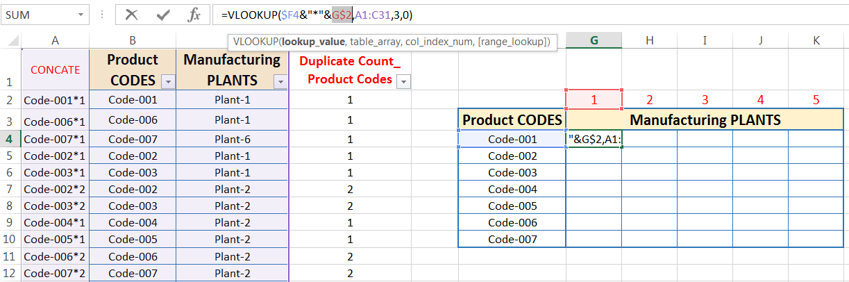
(iii). Select the range A1:C31 as a table_array with Ctrl+Shift+Right Arrow (➡) and Ctrl+Shift+Down Arrow (⬇).
Cell A1 refers to the first cell of the lookup column, whereas cell C31 refers to the end cell of the required column.
More technically, column A refers to the ‘CONCATE‘ column (means lookup column) whereas column C refers to the ‘Manufacturing PLANTS‘ (means required column).
=VLOOKUP(F4&“*“&G2, A1:C31
Place a comma (,) to move to the next argument.
(iv). Put a value 3 as a column_index_number, the third argument of VLOOKUP. Column number 3 refers to EXCEL to move 3 columns at the right starting from the lookup column. It indicates ‘Manufacturing Plants’.
For example, the lookup column is Column A (refers to ‘CONCATE’ Column) and VLOOKUP retrieves data from the required column, i.e., Column C (refers to ‘Manufacturing PLANTS’) just 3 columns right considering column A.
=VLOOKUP(F4&“*“&G2, A1:C31, 3
Place a comma (,) to move to the next argument.
(05). As we find an exact match, so put 0 (zero) or False in place of range_lookup, the fourth argument of VLOOKUP.
=VLOOKUP(F4&“*“&G2, A1:C31, 3, 0)

• Step 8: Using Cell References
(i). This is an important section and considers the lookup_value of the VLOOKUP function.
At first, select the cell F4 and press the F4 key three times to convert from the relative cell reference to the mixed cell reference (where the absolute column but the relative row).
Thus, it seems to be $F4.
Then select the cell G2 and press the F4 key twice to convert it from the relative cell reference to the mixed cell reference (where the row becomes absolute but the column remains relative).
Thus, it seems to be G$2.
(ii) Then select the range A1:C31 as table_array, the second argument of the VLOOKUP function, and press the F4 key once to convert the range from the relative cell reference to the absolute cell reference.
Thus, the lookup_array looks like $A$1:$C$31.
So, while copying the formula horizontally (row-wise) or vertically (column-wise) in any direction, columns address and row number remain fixed means they do not change at all.
(iii) Press ‘Enter’ to accept the changes in the formula.
Then the formula seems to be:
=VLOOKUP($F4&“*“&G$2, $A$1:$C$31, 3, 0)
• Step 9: Replacing Errors with the IFERROR function
The IFERROR function is a logical function which returns a value if a formula evaluates to an error; otherwise, it returns the result of the formula.
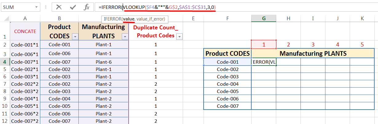
The syntax for the IFERROR function is
• value is a cell reference or formula.
• value_if_error is the message to be displayed if the value argument returns an error. We replace these errors with a character (such as space “ ” or zero 0 or any text within a double quotation mark, for example, “No value”) a snap. If Excel does not detect an error, the value is displayed as a result.
➢ Steps to Start:
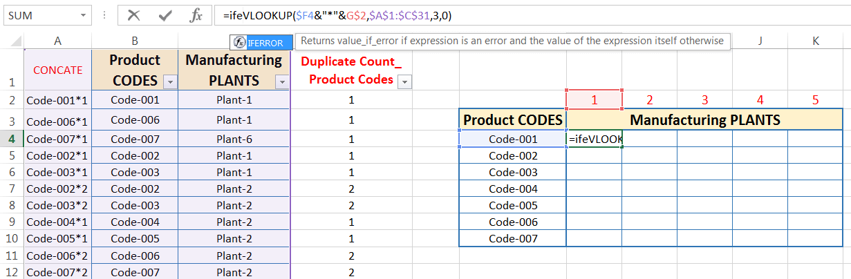
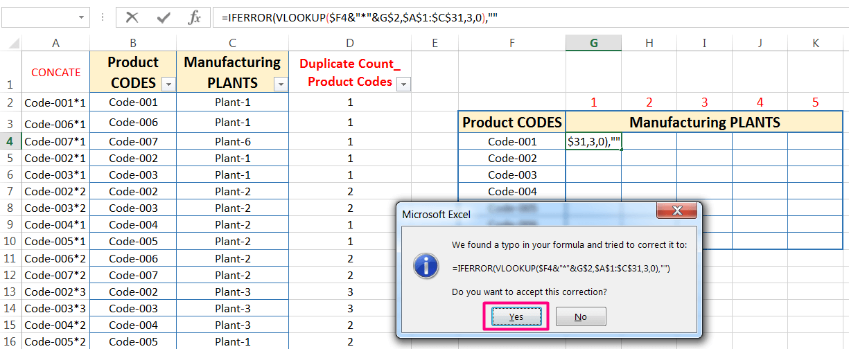
Edit the VLOOKUP formula in cell G4, we place the IFERROR function at the starting of the VLOOKUP formula. After the VLOOKUP formula place a comma (,). As a result, the entire VLOOKUP formula considers a value argument. After the placing comma, move to the next argument value_if_error where we use space (“ ”) as a character.
As a result, if the VLOOKUP function returns the error value #N/A, the second argument in the IFERROR function is executed, and space (“ ”) is displayed.
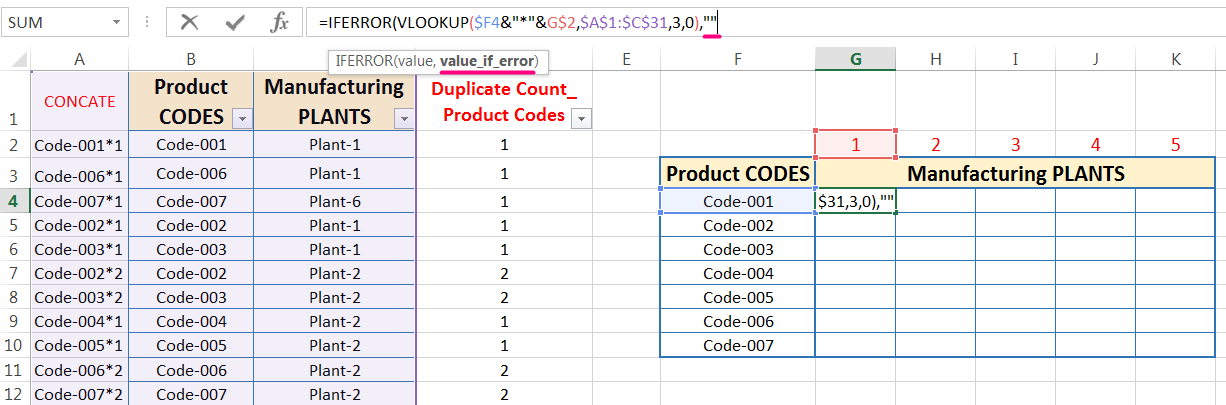
Press ‘Enter’ before the closing of parenthesis and Excel returns a warning message “We found a typo in your formula and tried to correct it to:”, either we press ‘Enter’ or click ‘Yes’ to accept this correction. EXCEL by default closes the last parenthesis and returns the result.
Then the formula seems to be:
=IFERROR(VLOOKUP($F4&“*“&G$2, $A$1:$C$31, 3, 0),” “)
Close the last parenthesis and press ‘Enter‘ to accept the formula.
Please note that before closing the last parenthesis, if we press ‘Enter‘ then Excel by default closes the last parenthesis.
• Step 10: Extending the Formula to the Entire Ranges: Alt+E+S+R / Alt+Ctrl+V+R
After getting the result, copy the cell G4 with Excel shortcut Ctrl+C ➪ making a selection of the entire ranges with Shift+ Right arrow (➡), Down arrow (⬇ ) ➪ press sequentially Alt+E+S+R (such as Alt, E, S, R) / Alt+Ctrl+V+R (such as Alt+Ctrl+V, R) which will select the option ‘Formulas and number formats‘ under the ‘Paste Special’ dialog box ➪ click on ‘OK’ or press ‘Enter’ to accept the formula.
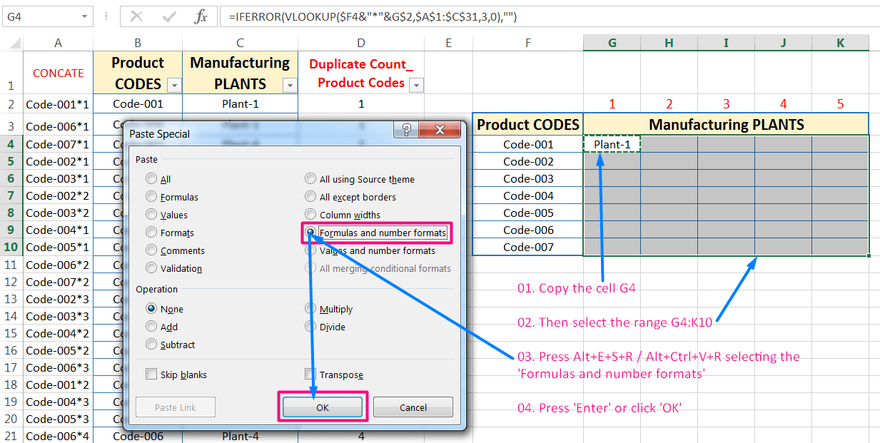
Note: Excel displays an animated marquee around cells that have been cut or copied. After pasting the contents to their new location cancel the animated marquee by pressing the ‘Esc‘ (Escape) key.


Join Our Community List
Subscribe to our mailing list and get interesting stuff and updates to your email inbox.