Multiple Columns VLOOKUP in Excel is an advanced level of the VLOOKUP formula where the formula is used once with a certain condition(s) in a cell and that allow retrieving matched data from a table/dataset, but after stretching the formula to the right-side (row-wise; horizontally) or down-side (column-wise; vertically) it works dynamically to retrieves data from the table against the matched criteria.

In the Corporate Sector, the common term of Multiple Columns Vlookup is Multiple VLOOKUP or Multiple LOOKUP or Matrix LOOKUP or VLOOKUP Multiple Columns.

Remember that, sometimes it makes a confusion between Multiple Criteria VLOOKUP and Multiple Columns VLOOKUP.

[ Table/ Dataset is a structured range that contains related data organized in row(s) or column(s) in a worksheet that increases the capability to manage and analyze information.] 

I. Basic Criteria of Multiple Columns VLOOKUP in Excel

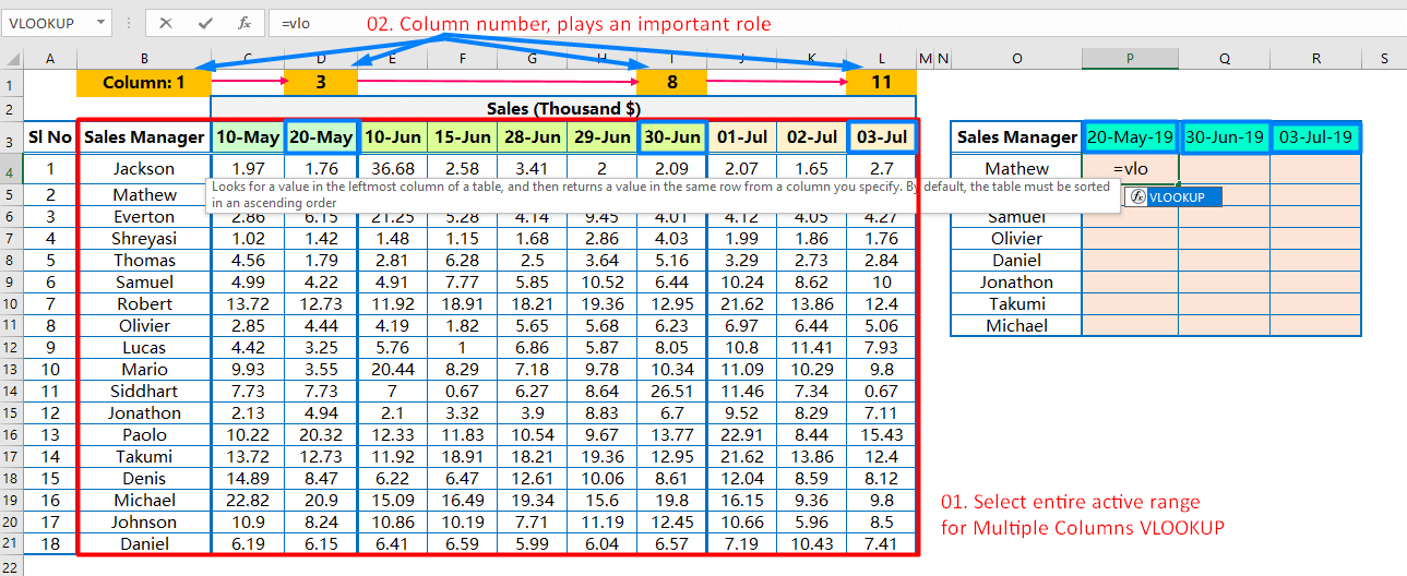
➢ Firstly, we select the entire database area (range) means entire table_area or table_array. More clearly, the area between the lookup column and the last column of the active database.

As a result, the selection range should not be expanded or diminished every time, need to change column number or column_index_num only.

➢ Secondly, we try out to make the column number or column_index_num to be dynamic.

➢ Thirdly, proper use of cell reference (relative, absolute, mixed) within first three VLOOKUP arguments (i.e., lookup_value, table_array, col_index_num). It makes a big sense to make a dynamic VLOOKUP formula.  Otherwise, the VLOOKUP formula returns an error.

II. Methods of Multiple Columns VLOOKUP in Excel

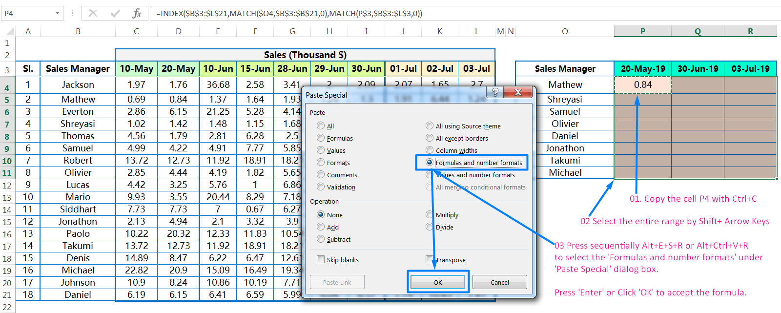
A single VLOOKUP formula with certain parameters is used to retrieve values/data from a table/dataset. In the following example, based on the list in cells A3:L21, to find out the sales value in cell P4 against the Sales Manager name mentioned in cell O4 and Sales Date mentioned in cell P3.

➢ Select cell P4 by clicking on it or press F2 key or via the formula bar.

➢ Assign the VLOOKUP formula or the INDEX formula.

➢ Press Enter to apply the formula in cell P4.

➢ Using cell references (relative, absolute, and mixed according to the requirement).

➢ Then copy (Ctrl+C) the cell P4 with formula and extends it to the right-side and down-side till the end of the range i.e., P4:R11.

Here we discuss 4 methodologies of Multiple Columns VLOOKUP or Multiple VLOOKUP in Excel:

(01) Simple Method: Needs to change the column_index_number manually.

(02) Advanced Method: Using the predefined Column number(s) and Cell References, making the dynamic formula.

(03) Matrix Method: Using the VLOOKUP and MATCH nested functions, making the dynamic formula.

(04) Matrix Method: Using the INDEX, MATCH and MATCH nested functions, making the dynamic formula.

(01) Simple Method: Needs to Change the column_index_number Manually

➢ Step1: For a basic understanding of Multiple Columns VLOOKUP or Multiple VLOOKUP in Excel, we go through the Simple Method at the beginning where the column number needs to change manually.

Cells range A3: L21 is the main database or master database. We retrieve data from this master database with the VLOOKUP formula.

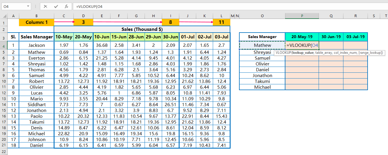
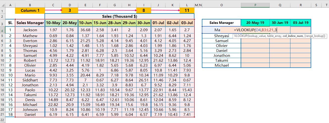
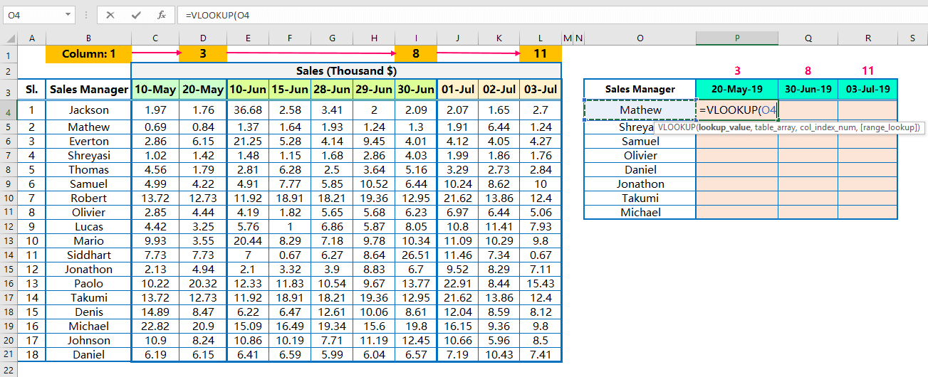
Place an equality sign (=) in cell P4 and type ‘VLO…’, select VLOOKUP from the below suggestion list of Down Arrow key (⬇), and press the ‘Tab’ key. VLOOKUP syntax appears with an open parenthesis.

Note: the upper or lower case does not matter in syntax, Excel by default considers it in upper case.

At first, we want to retrieve the sales value against Sales Manager Mathew on dated 20-May-19. Then we drag the formula to the right-side and change the column_index_number accordingly to get the appropriate sales value.

As the column_index_number plays an important role in Multiple Columns VLOOKUP, so we count the columns manually between the lookup column and the result column. For example,

(i) For the first instance, the lookup column is Column B i.e., the column with Sales Manager. Whereas, the result column (retrieve column) is column D which contains the sales values on 20-May-2019. The number of columns between Column B and D is 3.

(ii) Similarly, for the second instance, the lookup column is Column B and the result column is Column I (i.e., 30-Jun-19). The difference between Column B and I is 8.

(iii) Similarly, for the third instance, the lookup column is Column B and the result column is Column L (i.e., 03-Jul-19). The difference between Column B and L is 11.

➢ Step 2: Select the cell O4 as lookup_value, the first argument of VLOOKUP. Cell O4 refers to the Sales Manager ‘Mathew’.

Then place a comma (,) moving to the next argument.

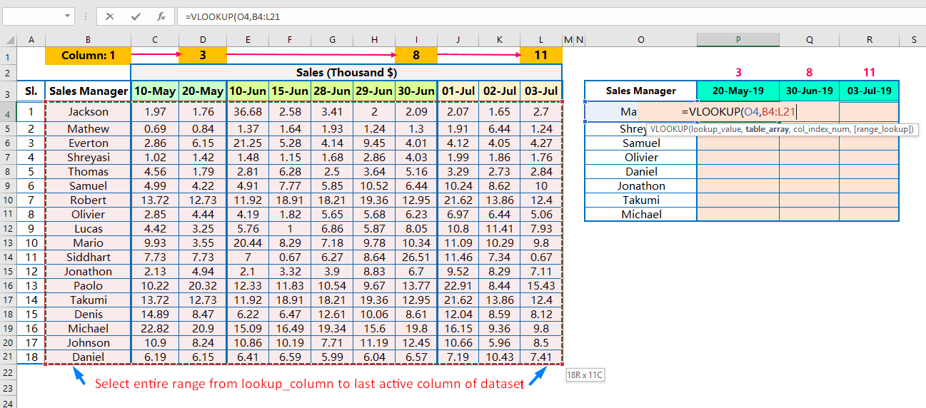
➢ Step 3: As discussed, select the entire range as table_array i.e., the range is B3:L21. B3 is the staring cell of the table and L21 is the last cell as well. That means, column B is the first column of the table and Column L is the last column in the table (or dataset).

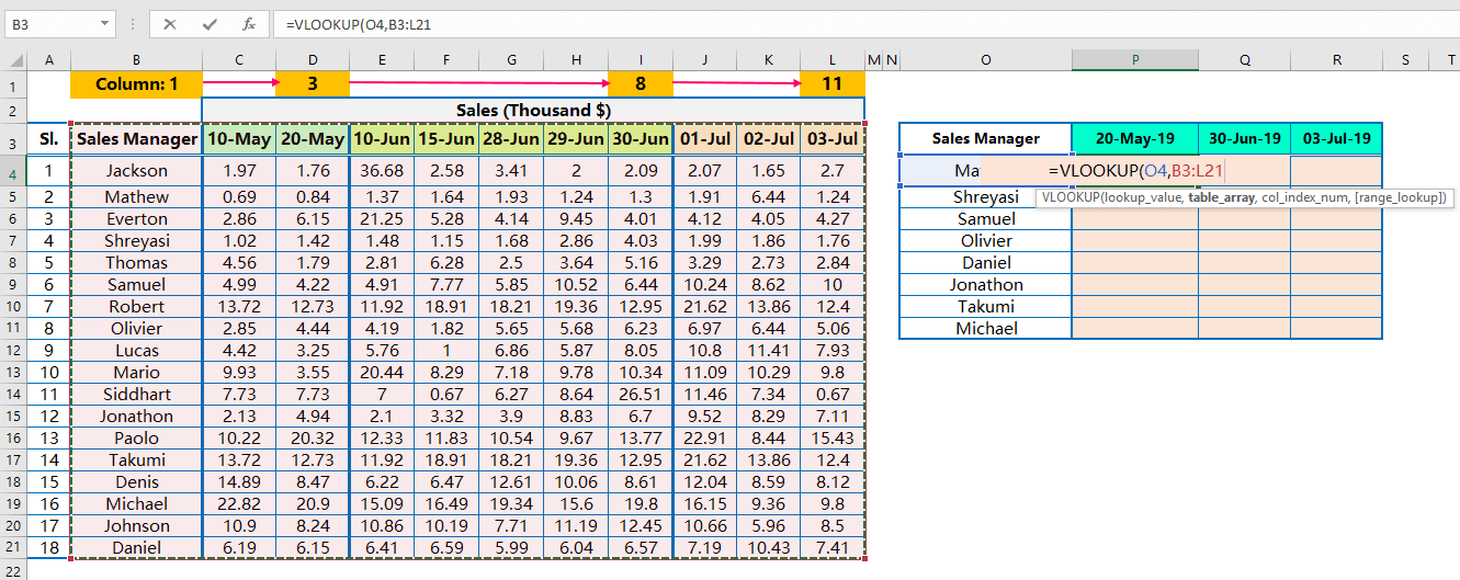
Why we select column B instead of column A? Because lookup values (i.e., Names of Sales Manager) are located in column B instead of column A.

Place a comma (,) to move to the next argument.

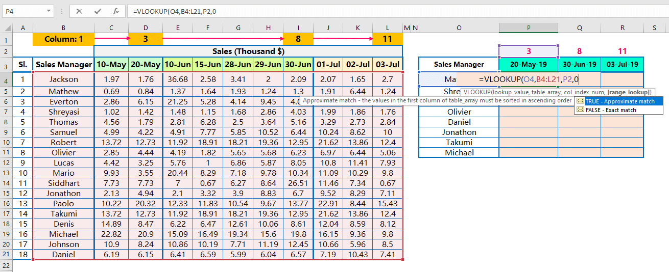
➢ Step 4: Put a value 3 as a column_index_number, the third argument of VLOOKUP. Column number 3 refers to EXCEL to move 3 columns right starting from the lookup column.

For example, the lookup column in our database is Column B and Excel retrieves data from Column D, just 3 columns right considering column B.

Place a comma (,) to move to the next argument.

➢ Step 5: As we find an exact match, so put 0 (zero) or False in place of range_lookup, the fourth argument of VLOOKUP.

➢ Step 6: Using of Cell References

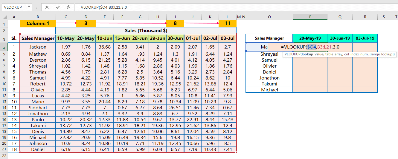
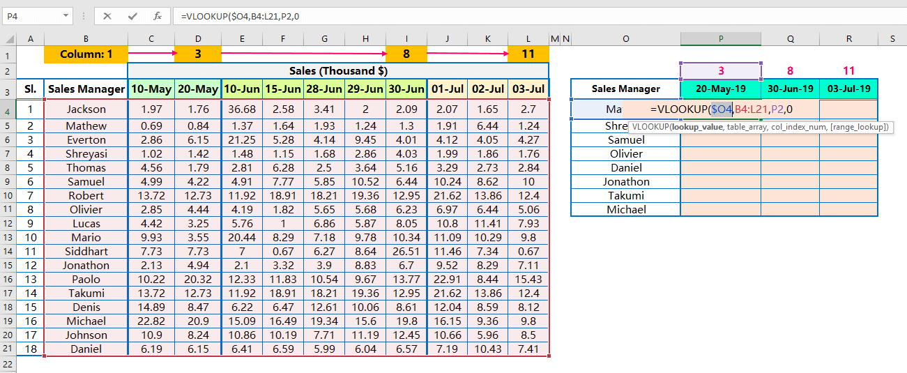
(i) This is an important section. At first, select the lookup_value and press F4 Key three times to convert from the relative cell reference to the mixed cell reference (where the column becomes absolute but the row remains relative).

Thus, it seems like $O4.

So in that case, when we copy the formula vertically (column-wise), the column addresses remain fixed, but row numbers simultaneously changed, like $O4, $P4, $Q4, $R4… so on.

(ii) Next, select the table_array and press F4 Key once to convert the range from the relative cell reference to the absolute cell reference.

Thus, the table_array seems to be $B$3:$L$21.

As a result, while copying the formula horizontally (row-wise) or vertically (column-wise) in any direction, columns address and row number do not change at all.

➢ Step 7: Finally, press ‘Enter’ to apply the formula in cell P4 and get the value as a result.

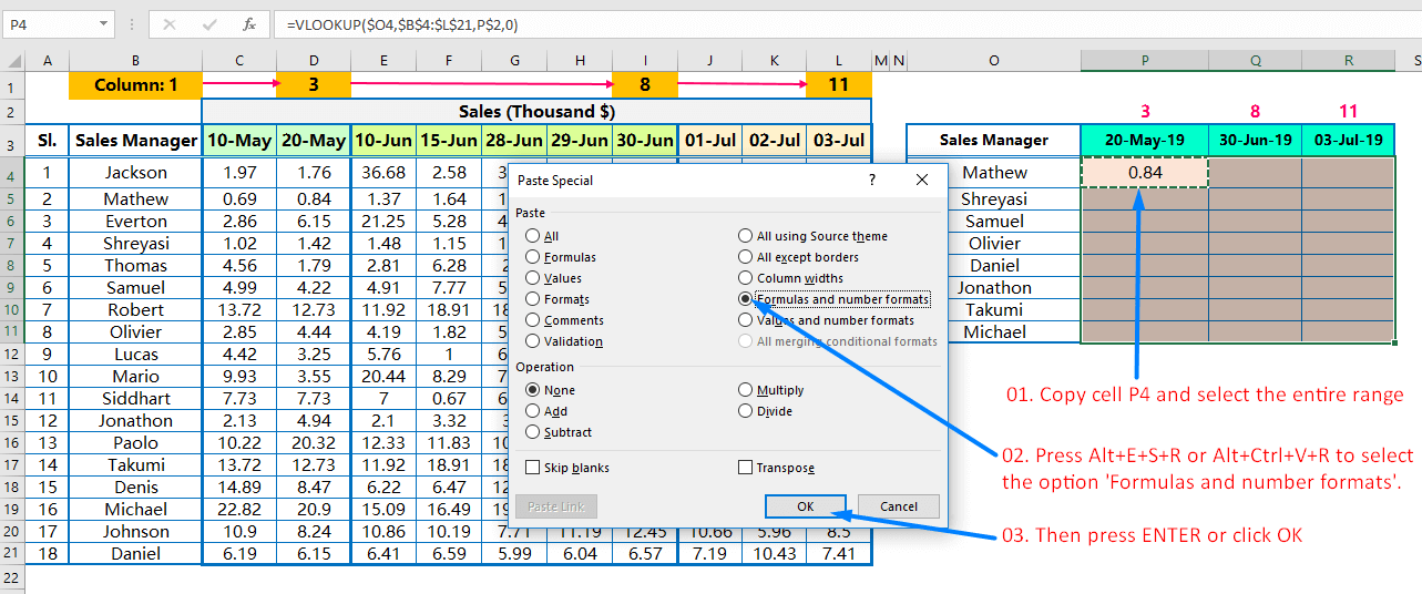
➢ Step 8: Extending the formula to the Right-Side (Row-Wise or Horizontally): Alt+E+S+R / Alt+Ctrl+V+R

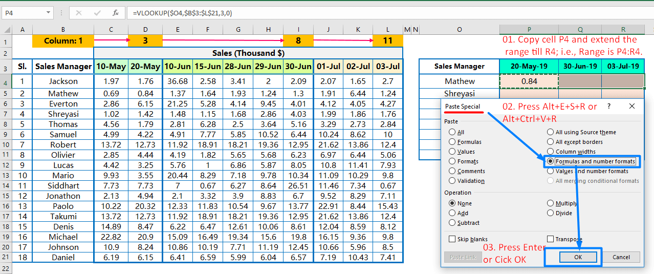
Copy (Ctrl+C) the cell P4 with formula and extends the selection to the right-side (same row or horizontally) ➪ press Alt+E+S+R / Alt+Ctrl+V+R sequentially, which will select the ‘Formulas and number formats‘ option under the ‘Paste Special’ dialog box ➪ then click on ‘OK’ or press ‘Enter’.

➢ Step 9: After extending the formula to the right side, we found that the same value is copied in all cells because of the column_index_number does not change dynamically.

So in that case, we have to change the column_index_number manually.

Edit the cell Q4 under the month 30-Jun-19 via the formula bar or press F2 key or by clicking on it ➪ change the column_index_number from 3 to 8 ➪ press ‘Enter‘ to accept the formula ➪ will get the correct result (figure as below).

Similarly, edit the cell R4 under the month 03-Jul-19 via the formula bar or press F2 key or by clicking on it ➪ change the column_index_number from 3 to 11 ➪ press ‘Enter‘ to accept the formula ➪ will get the correct result (figure as below).

➢ Step10: Extending the Formula to the Entire Range: Alt+E+S+R / Alt+Ctrl+V+R

After making changes, copy the range P4:R4 with Excel shortcut Ctrl+C ➪ then select the entire range P4:R11 with Shift+ Arrow Key(s) ➪ after that, press sequentially Alt+E+S+R / Alt+Ctrl+V+R which will select the option ‘Formulas and number formats‘ under the ‘Paste Special’ dialog box ➪ Click on ‘OK‘ or press ‘Enter‘ to accept the formula. 

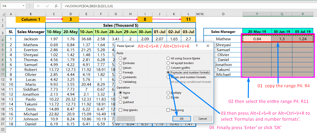
Finally, we retrieve the desired values from multiple columns against the matched criteria by using a single VLOOKUP. This is called Multiple Columns VLOOKUP or Multiple VLOOKUP, a special feature of VLOOKUP.

Press the ‘Esc’ (Escape) key to cancel the copy command.

■ Merits of this Simple Method for performing Multiple Columns VLOOKUP in Excel:

Instead of using multiple times of VLOOKUPs, a single VLOOKUP can manage to retrieve values from different columns aginst the matched criteria. This method saves a lot of time of daily Excel users.

■ Demerits of this Simple Method:

Manually change the column_index_number every time when formula copied to other columns.

(02) Advanced Method: Using the Predefined Column number(s) & Cell References

In this section, we use an advanced method for performing the Multiple Columns VLOOKUP or Multiple VLOOKUP in Excel.

➢ Step 1: Before applying the VLOOKUP formula, need to mention the specific retrieving column number just above each column.

➢ Step 2: Place an equality sign (=) in cell P4 and type ‘VLO’, select VLOOKUP from the below suggestion list by Down Arrow key (⬇) and then press the ‘Tab’ key. VLOOKUP syntax appears with an open parenthesis.

Then, Select the cell O4 as lookup_value, the first argument of VLOOKUP. Cell O4 refers to the name of a Sales Manager ‘Mathew’.

Place a comma (,) to move to the next argument.

➢ Step 3: Select the entire range (B4:L21 or B3:L21) as table_array i.e., start from the first cell of the lookup column (B3 or B4) to the end cell of an active dataset (L21).

Place a comma (,) to move to the next argument.

➢ Step 4: Now select the col_index_num as cell P2 (where we already mentioned the retrieve column number), the third argument of VLOOKUP. Follow the below figure:

Place a comma (,) to move to the next argument.

➢ Step 5: As we find an exact match, so put 0 (zero) or False in place of range_lookup, the fourth argument of VLOOKUP.

➢ Step 6: Using of Cell References

(i) This is an important section. At first, select the lookup_value and press F4 Key three times to convert from the relative cell reference to the mixed cell reference (where the absolute column but the relative row).

Thus, it seems like $O4.

So in that case, when we copy the formula vertically (column-wise), the column addresses remain fixed, but row numbers simultaneously changed, like $O4, $P4, $Q4, $R4… so on.

(ii) Next, select the table_array and press F4 Key once to convert the range from the relative cell reference to the absolute cell reference.

Thus, the table_array seems to be $B$4:$L$21 or $B$3:$L$21 (according to the selection of the range).

As a result, while copying the formula horizontally (row-wise) or vertically (column-wise) in any direction, columns address and row number do not change at all.

(iii)  After that, select the col_index_num (i.e., column_index_number) and press F4 Key twice to convert it from the relative cell reference to the mixed cell reference (where the row becomes absolute but the column remains relative).

Thus, it seems like P$2.

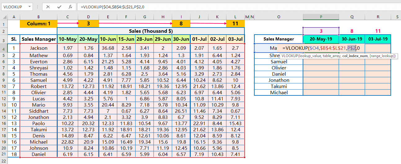
So in that case, while copying the formula horizontally (row-wise), the row numbers remain fixed, but column addresses simultaneously changed, like P$2, Q$2, R$2, S$2 …so on.

➢ Step 7: Finally, press ‘Enter‘ to apply the formula in cell P4 and get the value as a result.

➢ Step 8: Extending the Formula to the Entire Range: Alt+E+S+R / Alt+Ctrl+V+R

After getting the result, copy the cell P4 with Excel shortcut Ctrl+C ➪ making a selection of the entire range with Shift+ Right arrow (➡),  Down arrow (⬇ ) ➪ press sequentially Alt+E+S+R / Alt+Ctrl+V+R which will select the option ‘Formulas and number formats‘ under the ‘Paste Special’ dialog box ➪ Click on ‘OK’ or press ‘Enter’ to accept the formula.

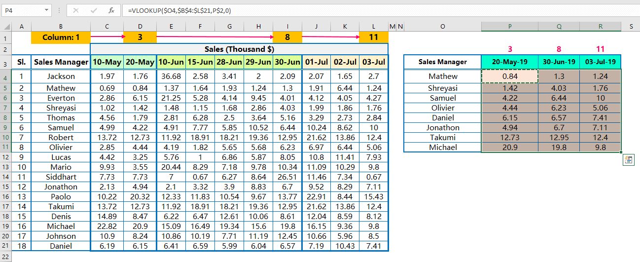
Finally, we get the required values from multiple columns against the matched criteria by using a single VLOOKUP. This is an example of advanced Multiple Columns VLOOKUP or advanced Multiple VLOOKUP. 

Press the ‘Esc’ (Escape) key to cancel the copy command.

■  Note:

We can formulate column numbers with the MATCH() function. The Syntax of the MATCH() function is:

But two things must remember before applying the formula:

(i)  Lookup_array should start from the lookup column. In the given example, lookup_array is B3:L3. Column B is the lookup column of VLOOKUP. Column L is the last column of the active dataset/table. 

(ii) Please keep in mind that there should not be any duplicate subject headings. If there is any duplicity in headings criteria, the MATCH function only retrieves the value against first matched criteria. 

■  Merits of this Advanced Method for performing Multiple Columns VLOOKUP:

1. This method saves a lot of time for daily Excel users in Corporate sectors, especially where need to consolidate multiple files from different users and system dump on a daily basis.  

2. No need for the subject heading.

3. No effect on duplicate subject headings, because we mention a specific column number on each case to retrieve data. This column number defines a specific column. So there has no relation with duplicate subject headings. 

(03) Matrix Method: Using the VLOOKUP & MATCH Nested Functions

In this section, VLOOKUP MATCH nested function allows performing Multiple Columns VLOOKUP or Multiple VLOOKUP in Excel. As this method performs a 2D lookup (two-dimensional lookup), so this method is called the Matrix Method.

➢ Step 1: In the first step, place an equality sign (=) in cell P4 and type ‘VLO...’ and press the ‘Tab’ key. VLOOKUP syntax appears with an open parenthesis.

Then, Select the cell O4 as lookup_value, the first argument of VLOOKUP. Cell O4 refers to the Sales Manager named by Mathew.

Place a comma (,) to move to the next argument.

➢ Step 2: Select the entire range (B3:L21) as table_array i.e., start from the first cell of the lookup column (B3) to the end cell (L21) of an active dataset/table.

Place a comma (,) to move to the next argument.

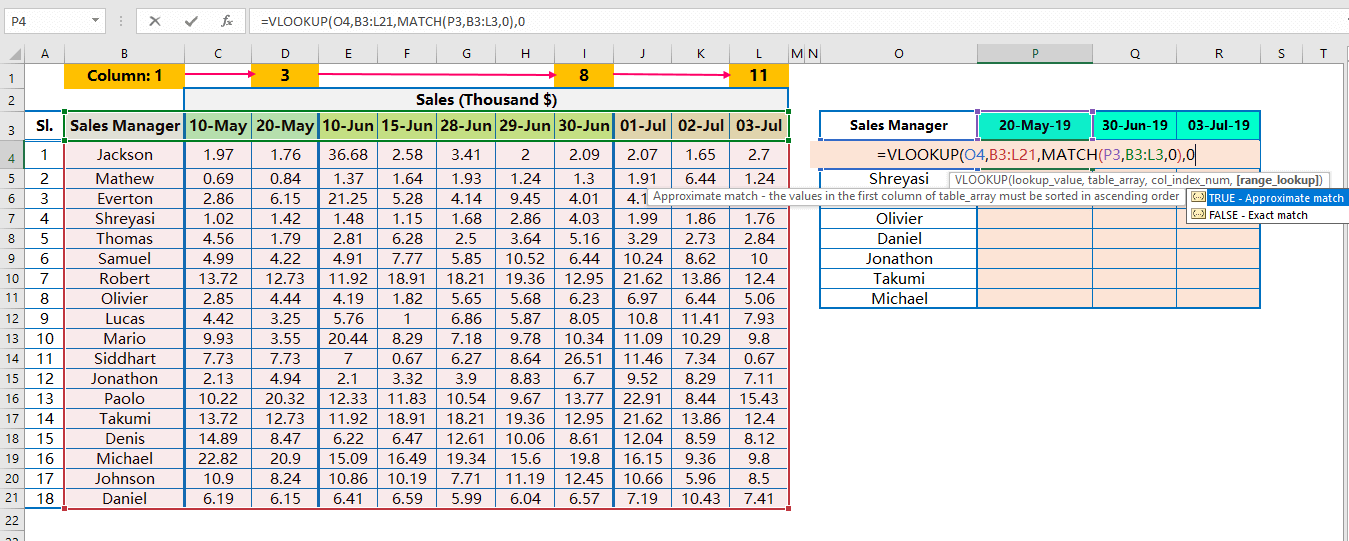
➢ Step 3: We use the MATCH() function in place of col_index_num of updating the column number automatically according to the change of a column, so the VLOOKUP formula works dynamically.

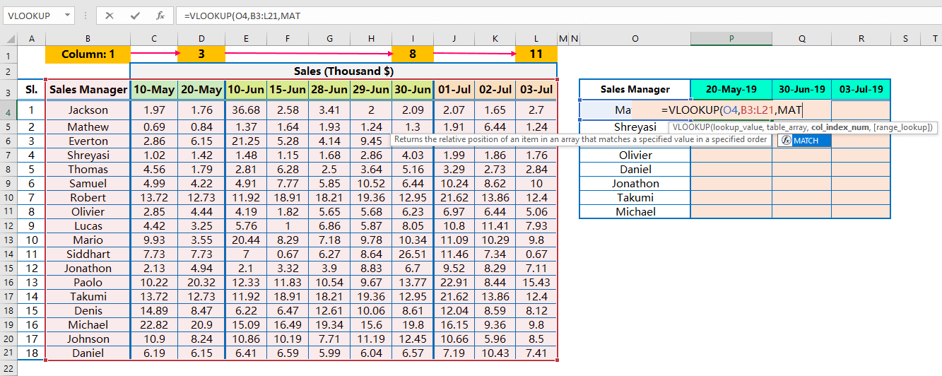
In place of the third argument, just type ‘MAT…’ and then press the ‘Tab’ key. MATCH syntax appears with an open parenthesis.

Within the MATCH function:

(i)  Select cell P3 as lookup_value, the first argument of MATCH() function. Cell P3 refers to a date, i.e., 20-May-19.

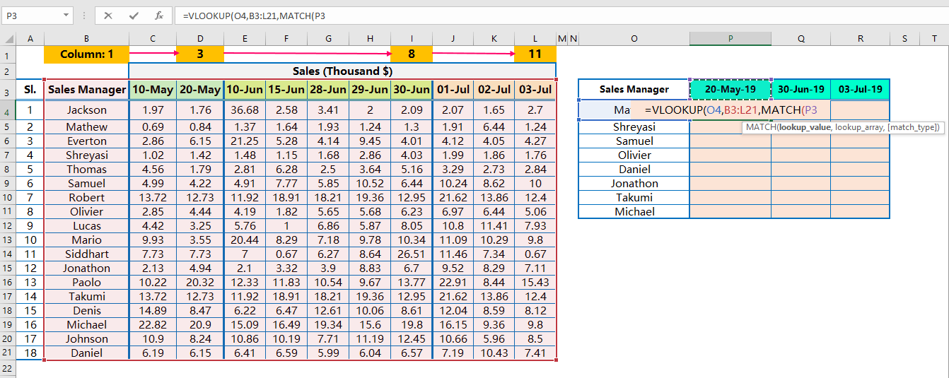
Place a comma (,) to move to the next argument.

(ii) Select the range B3:L3 as lookup_array, the second argument of MATCH() function.

Please keep in mind that the starting point (or starting column) of lookup_array should be the same as a lookup column of VLOOKUP. Column B is the lookup column of the VLOOKUP formula, that’s why we start the lookup_array from column B.

MATCH() function is a single array function that means it works only in a single row or in a single column. As per requirement, we select a single row (range is B3:L3) instead of selecting the entire range.

(iii) As we find an exact match, so put 0 (zero) or False in place of match_type, the third argument of MATCH() function.

Then close the fist parenthesis of the MATCH function and place a comma (,) moving to the last argument of the VLOOKUP function.

➢ Step 4: As we find an exact match, so put 0 (zero) or False in place of range_lookup, the fourth argument of VLOOKUP.

➢ Step 5: Using of Cell References

(i) First, select the lookup_value and press the F4 Key three times to convert from the relative cell reference to the mixed cell reference (where the column address is absolute but the row is relative).

Thus, it seems like $O4.

So in that case, while copying the formula vertically (column-wise), the column addresses remain fixed, but row numbers simultaneously changed, like $O4, $P4, $Q4, $R4… so on.

(ii) In the next step, select the table_array and press F4 Key once to convert the range from the relative cell reference to the absolute cell reference.

Thus, the table_array seems to be $B$3:$L$21.

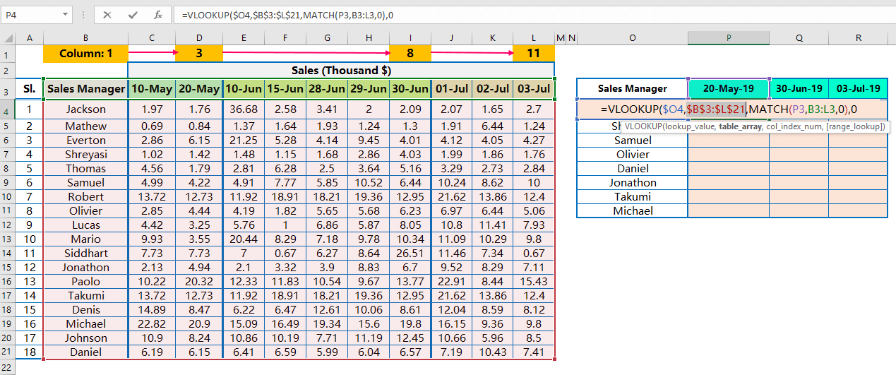
As a result, while copying the formula horizontally (row-wise) or vertically (column-wise) in any direction, columns address and row numbers do not change at all.

(iii)  Then, select the col_index_num (i.e., column_index_number) where the MATCH function has applied.

(a) Select the cell P3 as lookup_value, the first argument of MATCH function, and press the F4 Key twice to convert it from the relative cell reference to the mixed cell reference (where the row is absolute but the column address is relative).

Thus, it seems like P$3.

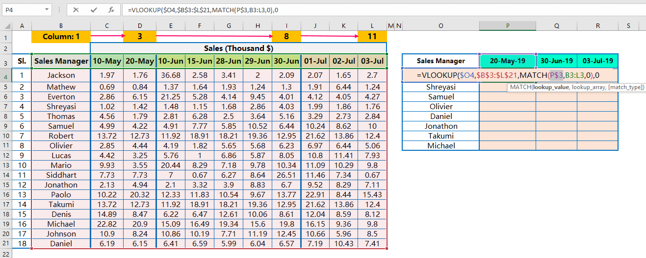
Thus, while copying the formula horizontally (row-wise), the row number remains fixed, but the column address simultaneously changed, like P$3, Q$3, R$3, S$3 …so on.

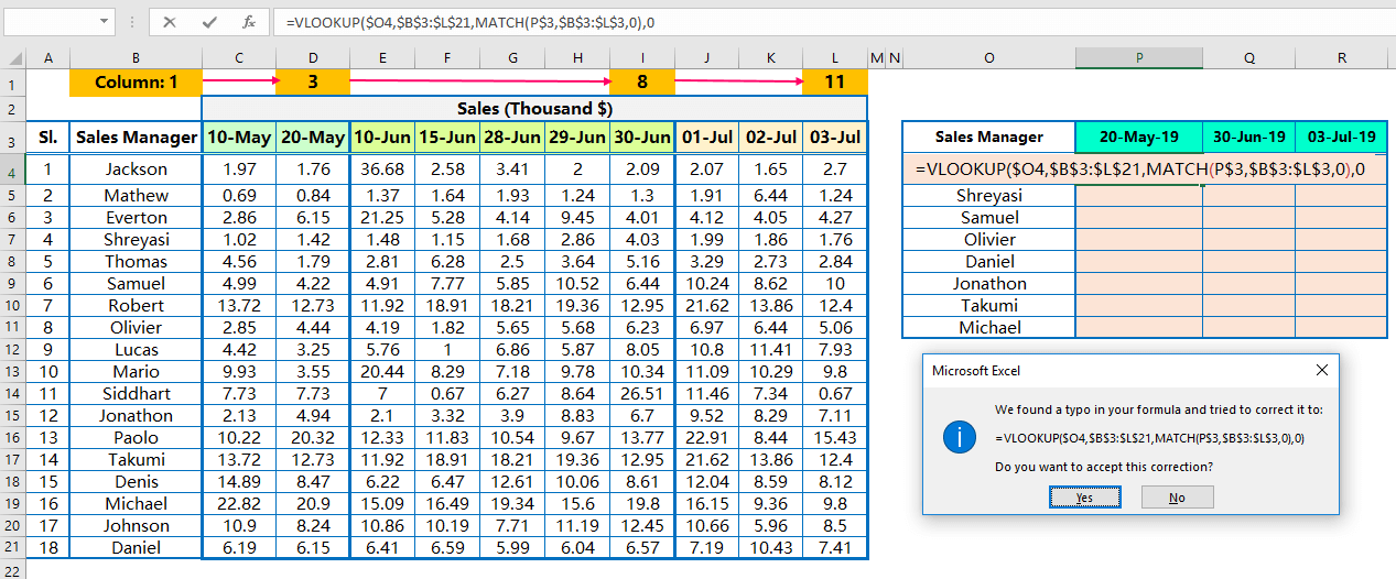
(b) Then select the range B3:L3 as lookup_array, the second argument of the MATCH function, and press the F4 key once to convert the range from the relative cell reference to the absolute cell reference.

Thus, the lookup_array looks like $B$3:$L$3.

So, while copying the formula horizontally (row-wise) or vertically (column-wise) in any direction, columns address and row number remain fixed means they do not change at all.

➢ Step 6: Finally, press Enter to apply the formula and Excel returns a warning message “We found a typo in your formula and tried to correct it to:”, either we press ‘Enter’ or click ‘Yes’ to accept this correction. EXCEL by default closes the last parenthesis and returns the result.

➢ Step 7: Extending the Formula to the Entire Range: Alt+E+S+R / Alt+Ctrl+V+R

This step is similar to before. After getting the result, copy the cell P4 with Excel shortcut Ctrl+C ➪ making a selection of the entire range with Shift+ Right arrow (➡),  Down arrow (⬇ ) ➪ press sequentially Alt+E+S+R / Alt+Ctrl+V+R which will select the option ‘Formulas and number formats‘ in the ‘Paste Special’ dialog box ➪ Click on ‘OK’ or press ‘Enter’ to accept the formula.

Finally, we get the desired values from multiple columns against the matched criteria with the help of a single VLOOKUP.

Press the ‘Esc’ (Escape) key to cancel the copy command.

■ Merits of the VLOOKUP MATCH Matrix Lookup Method:

1. This method also saves a lot of time for daily Excel users.

2. No need for the subject heading.

3. There is an effect of duplicate headings, as MATCH() function is used. So keep notice of that. 

(04) Matrix Method: Using the INDEX, MATCH & MATCH Nested Functions

INDEX, MATCH and MATCH functions cumulatively make a nested formula which is the best alternative of Multiple Columns VLOOKUP or Multiple Lookup in Excel. This method performs a 2D lookup (two-dimensional lookup), so this method is called the Matrix Method.

The INDEX function returns a specific value or the address of a specific value from within an array, table, or range.

➢ The Syntax for the INDEX Function

The INDEX function’s arguments are as follows:

• array: A range

• row_num: A row number within the array

• col_num: A column number within the array

The INDEX function always returns a value specified by the intersection of the row_number and column_number. If the array is one dimensional, meaning it contains a single row per column, then both row_num  and column_num are not required.

The INDEX function is more frequently used with two-dimensional array or tables.  

The MATCH and INDEX functions are often used together to perform lookups. The MATCH function returns the relative position of a cell in a range that matches a specified value.

➢ The Syntax for the MATCH Function

The MATCH function’s arguments are as follows:

• lookup_value: The value that matches in lookup_array. If match_type is 0 and the lookup_value is text, this argument can include wildcard characters asterisk (*) and question mark (?).

• lookup_array: The range being searched.

• match_type: An integer (-1, 0, or 1) that specifies how the match is determined.

If match_type is 1, MATCH finds the largest value less than or equal to lookup_value. (lookup_array must be in ascending order.)

If match_type is 0, MATCH finds the first value exactly equal to lookup_value.

 If match_type is -1, MATCH finds the smallest value greater than or equal to lookup_value. (lookup_array must be in descending order.) If we omit the match_type argument, this argument is assumed to be 1.

➢ The Syntax for the INDEX, MATCH & MATCH Nested Function

➢ Step to Start

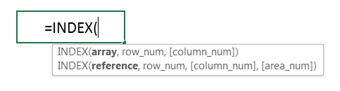
• Step 1: In the first step, place an equality sign (=) in cell P4 and type ‘ind…’, select INDEX by down arrow (if required), and press the ‘Tab’ key. INDEX syntax appears with an open parenthesis.

Then, select the range B3:L21 as an array, the first argument of the INDEX function.

Please keep in mind that we should take more attention to range selection. For example, here we select range B3:L21 instead of A3:L21. Because column B is the lookup_column where criteria exist. The cell B3 is the starting point or starting cell for the MATCH function.

Place a comma (,) to move to the next argument.

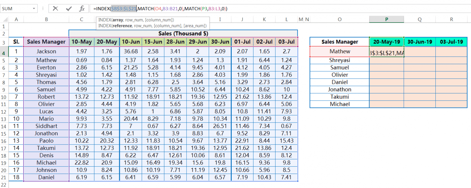
• Step 2: We use the first MATCH() function in place of row_num, the second argument of INDEX function, getting the row number against the matched criteria.

In this case, just type ‘MAT…’ and then press the ‘Tab’ key. MATCH syntax appears with an open parenthesis.

Within the MATCH function:

(i)  Select cell O4 as lookup_value, the first argument of MATCH() function. Cell O4 refers to the Sales Manager named by ‘Mathew’.

Place a comma (,) to move to the next argument.

(ii) Select the range B3:B21 as lookup_array, the second argument of MATCH() function.

As discussed above, the cell B3 is the starting point (or starting column or lookup column) of the INDEX function and MATCH function(s) as well.

MATCH() function is a single array function that means it works only in a single row or in a single column. As row_number is required for the second argument of the INDEX function, we select a single column (range is B3:B21) instead of selecting a row or the entire range.

(iii) As we find an exact match, so put 0 (zero) or False in place of match_type, the third argument of MATCH() function.

Then close the fist parenthesis of the MATCH function and place a comma (,) moving to the third argument of the INDEX function.

• Step 3: Then we use the second MATCH() function in place of column_num, the third argument of the INDEX function, getting the column number against the matched criteria.

In this case, just type ‘MAT…’ and then press the ‘Tab’ key. MATCH syntax appears with an open parenthesis.

Within the MATCH function:

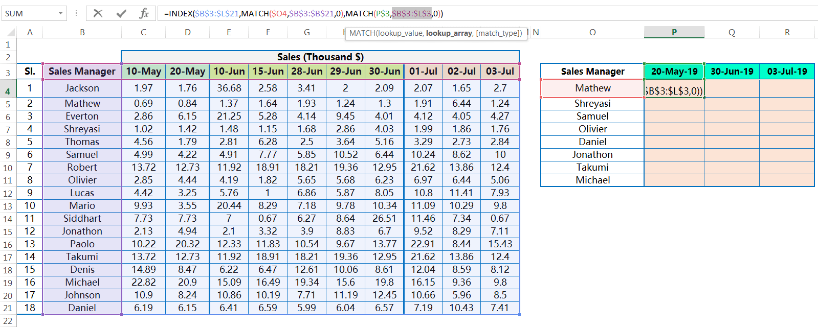
(i)  Select cell P3 as lookup_value, the first argument of MATCH() function. Cell P3 refers to a date, i.e., 20-May-19.

Place a comma (,) to move to the next argument.

(ii) Select the range B3:L3 as lookup_array, the second argument of MATCH() function.

As discussed above, the cell B3 is the starting point (or starting column or lookup column) of the INDEX function and MATCH function(s) as well.

MATCH() function is a single array function that means it works only in a single row or in a single column. As column_number is required for the third argument of the INDEX function, we select a single row (range is B3:L3) instead of selecting a column or the entire range.

(iii) As we find an exact match, so put 0 (zero) or False in place of match_type, the third argument of MATCH() function.

• Step 4: Finally, close the first parenthesis of the MATCH function and the INDEX function as well. Then press ‘Enter’ to accept the formula.

Otherwise, before closing the parentheses press ‘Enter’ to accept the formula and Excel returns a warning message “We found a typo in your formula and tried to correct it to:”, either we press ‘Enter’ or click ‘Yes’ to accept this correction. EXCEL by default closes the last parentheses and returns the result.

• Step 5: Using of Cell References

(01) First, select the index_array and press the F4 Key once to convert the range from the relative cell reference to the absolute cell reference.

Thus, the array seems to be $B$3:$L$21.

As a result, while copying the formula horizontally (row-wise) or vertically (column-wise) in any direction, columns address and row number remain fixed means they do not change at all.

(02) Then move into the first MATCH function.

(a) Select the cell O4 as lookup_value, the first argument of the MATCH function, and press the F4 key three times to convert it from the relative cell reference to the mixed cell reference (where the column address is absolute but the row number is relative).

Thus, it seems like $O4.

Thus, while copying the formula vertically (column-wise), the column address remains fixed, but the row number simultaneously changed, like $O4, $O5, $O6, $O7 …so on.

(b) Then select the range B3:B21 as lookup_array, the second argument of MATCH function, and press the F4 key once to convert the range from the relative cell reference to the absolute cell reference.

Thus, the lookup_array seems to be $B$3:$B$21.

So, while copying the formula horizontally (row-wise) or vertically (column-wise) in any direction, columns address and row number remain fixed means they do not change at all.

(03) Then move into the Second MATCH function.

(a) Select the cell P3 as lookup_value, the first argument of MATCH function, and press F4 Key twice to convert it from the relative cell reference to the mixed cell reference (where the row is absolute but the column address is relative).

Thus, it seems like P$3.

Thus, while copying the formula horizontally (row-wise), the row number remains fixed, but the column address simultaneously changed, like P$3, Q$3, R$3, S$3 …so on.

(b) Then select the range B3:L3 as lookup_array, the second argument of MATCH function, and press the F4 key once to convert the range from the relative cell reference to the absolute cell reference.

Thus, the lookup_array looks like $B$3:$L$3.

So, while copying the formula horizontally (row-wise) or vertically (column-wise) in any direction, columns address and row number remain fixed means they do not change at all.

(04) Press ‘Enter’ to accept the formula.

• Step 6: Extending the Formula to the Entire Range: Alt+E+S+R / Alt+Ctrl+V+R

This step is similar to before. After getting the result, copy the cell P4 with Excel shortcut Ctrl+C ➪ making a selection of the entire range with Shift+ Right arrow (➡),  Down arrow (⬇ ) ➪ press sequentially Alt+E+S+R / Alt+Ctrl+V+R which will select the option ‘Formulas and number formats‘ under the ‘Paste Special’ dialog box ➪ Click on ‘OK’ or press ‘Enter’ to accept the formula.

Finally, we get the desired values from multiple columns against the matched criteria with the help of a Matrix lookup (INDEX, MATCH, and MATCH nested function).

Press the ‘Esc’ (Escape) key to cancel the copy command.

■ Merits of the INDEX MATCH Matrix Lookup Method:

This is the best alternative of the VLOOKUP MATCH Matrix Lookup method for performing Multiple Columns VLOOKUP in Excel.