


(A). WHAT IS EXCEL VLOOKUP FUNCTION?
The Excel VLOOKUP function is a lookup and reference function that accepts a value that looks the value up in a vertical lookup table with data organized in columns and returns a result. The Excel VLOOKUP function is one of the most popular Excel lookup functions.
More specifically, the Excel VLOOKUP signifies ‘vertical lookup‘ (The ‘V’ stands for ‘Vertical’) and it is an Advanced Excel function that searches for a value in the first column (more specifically, lookup column where lookup value exists) of the lookup table and looks up to the right and returns the corresponding value in the same row of a specified table column.
The lookup table is arranged in vertical columns (which explains the ‘V’ in the function’s name). Each column is used for a new record.
Excel VLOOKUP supports approximate match (indicated by ‘TRUE’ or numerical ‘1’), exact match (indicated by ‘FALSE’ or numerical ‘0’), and wildcard (such as asterisk ‘*‘, question mark ‘?‘) for partial matches.
(B). HOW TO USE EXCEL VLOOKUP FUNCTION?
in Advance Excel, The Excel VLOOKUP function is used in different ways:
- Using the VLOOKUP function to Find an Exact Match
- Using the VLOOKUP function to Find an Approximate Match
- Using the VLOOKUP function to Find a Partial Match
- The VLOOKUP function performing a ‘Left LOOKUP’ or ‘Reverse LOOKUP’
- The VLOOKUP function performing a ‘Double VLOOKUP’ or ‘Nested VLOOKUP’ or ‘IFERROR VLOOKUP’
- The VLOOKUP function performed with multiple criteria
- The VLOOKUP function performed with multiple columns
- The VLOOKUP function performed with multiple sheets
- The VLOOKUP function performed with Pivot Table
- The VLOOKUP function nested with COUNTIFS finds the duplicate entry
- The VLOOKUP function nested with the IF function performed logical VLOOKUP
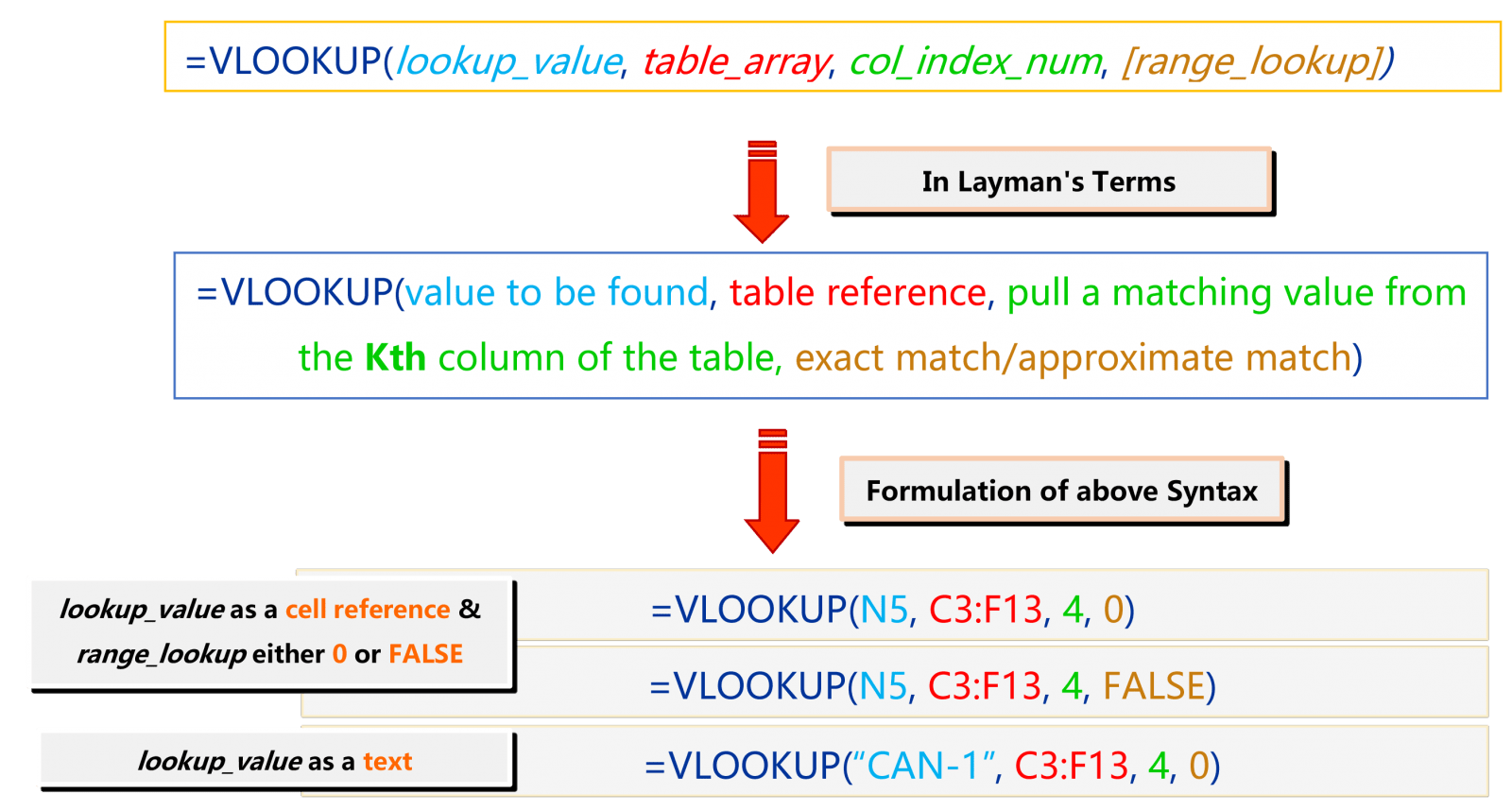
➢ THE SYNTAX FOR THE EXCEL VLOOKUP FUNCTION
➢ THE ARGUMENTS OF THE EXCEL VLOOKUP FUNCTION
There are 04 arguments in the Excel VLOOKUP function are as follows:
• lookup_value [Required Argument]
The specific value to be looked up in the lookup column (i.e., the first column) of the lookup table is called the lookup_value.
For example, if the lookup_value is located in cell C3 then our range should be started with column C; if the lookup_value present in any cell of column D (for example, D3, D4, D7, etc.), then the range should be started with column D.
Lookup_value can be either a value (number, date, or text) or a cell reference (a reference to a cell containing a lookup value), or the value returned by some other Excel function. For example:
(i) Lookup-value may be a value: =VLOOKUP(90, C3:F13, 4,0) – the formula will search for the number 90 (i.e., the lookup_value) in the range C3:F13. Please note that we don’t use “double quotes” for the numeric values.
(ii) Lookup-value may be a text: =VLOOKUP(“CAN-1“, C3:F13, 4,0) – the formula will search for the text “CAN-1” (i.e., the lookup_value) in the range C3:F13. Please note that we always enclose the text in “double quotes”.
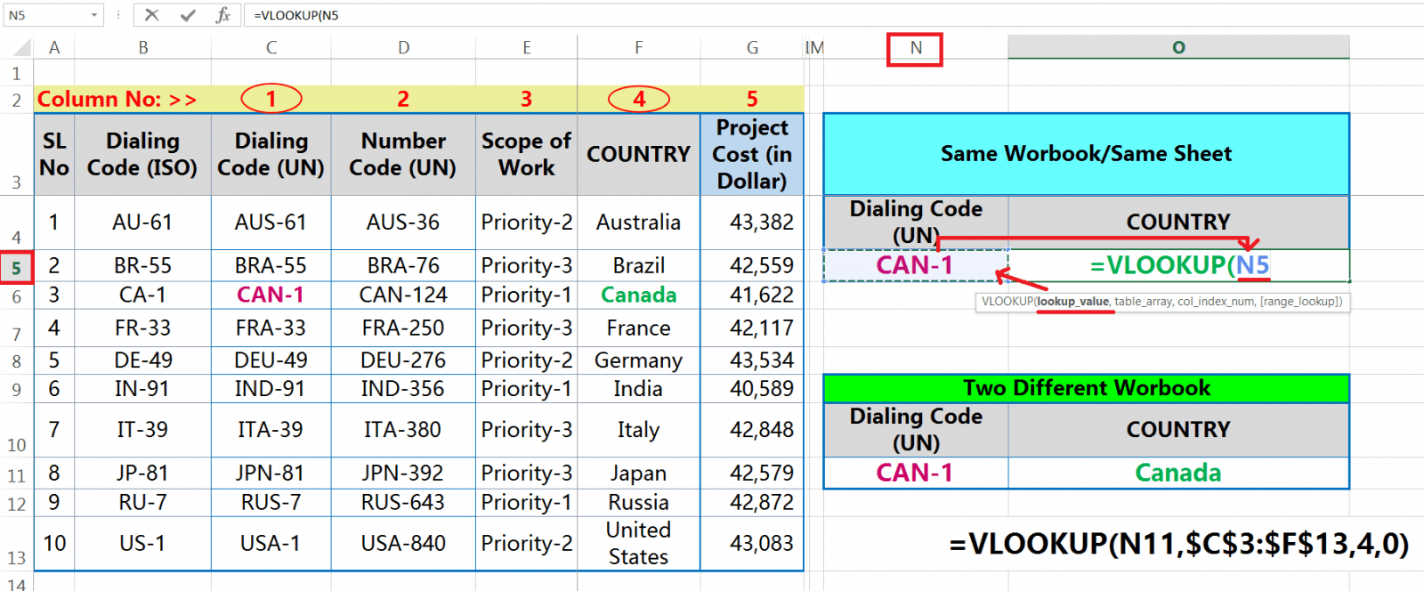
(iii) Lookup-value may be a cell reference: =VLOOKUP(N5, C3:F13, 4,0) – the formula will search for the value in cell N5 (i.e. ‘CAN-1’). N5 is the cell address of ‘CAN-1’. More specifically we can say N5 is the cell reference of ‘CAN-1’. Using the cell reference(s) in a formula makes the formula dynamic instead of manually typing a value.
• table_array [Required Argument]
The table_array is the range that contains one or more columns of the lookup table. It is basically the rectangular grid of cells that contains all the data we’re searching for retrieving a value.
The Excel VLOOKUP function starts searching from the leftmost column (i.e., the first column of the lookup table is also called the lookup column) of the table array. Always keep in mind that, first column / lookup_column starts from where the lookup value exists.
The Excel VLOOKUP function retrieves the value from the column in the table_array is called the result column. The lookup column and the result column may be the same (when selecting the single column) or different.
Thus, the Excel VLOOKUP formula =VLOOKUP(“CAN-1”, C3:F13, 4, 0) will search for the value “CAN-1” from a range of cells, i.e., C3 to F13 where column C is the first column or lookup column and column F is the result column of the lookup_array.
The table array may contain various values such as text, dates, numbers, or logical values. Values are case-insensitive, which means that uppercase and lowercase text are treated as identical.
So, we can write the Excel VLOOKUP formula in such a way =VLOOKUP(“can-1“, C3:F13, 4, 0). The lowercase “can-1” is symmetrical to the upper case “CAN-1”. As a result, the Excel VLOOKUP formula retrieves the same value right to the “CAN-1”.
This is very important that when the Excel VLOOKUP formula performs in the same workbook, the table array remains in the relative cell reference (which means there has no dollar $ sign), for example, C3:F13; whereas the Excel VLOOKUP formula performs in the different workbooks, the table array by default changes to an absolute cell reference (one dollar $ sign before the column address and another dollar $ sign before the row address), for example, $C$3:$F$13.

• col_index_num [Required Argument]
This is an integer / positive value. The col_index_num denotes the count of column numbers between the lookup column and the result column in the table_array from which the matching value is returned. Basically col_index_num starting from the lookup column and ends in the result column.
The lookup column, is the first column in the table_array, defines as 1, the second column is 2, the third column is 3, and so on till the result column. Sometimes, the lookup column and the result column can be the same, so in this case, col_index-num defines as 1.
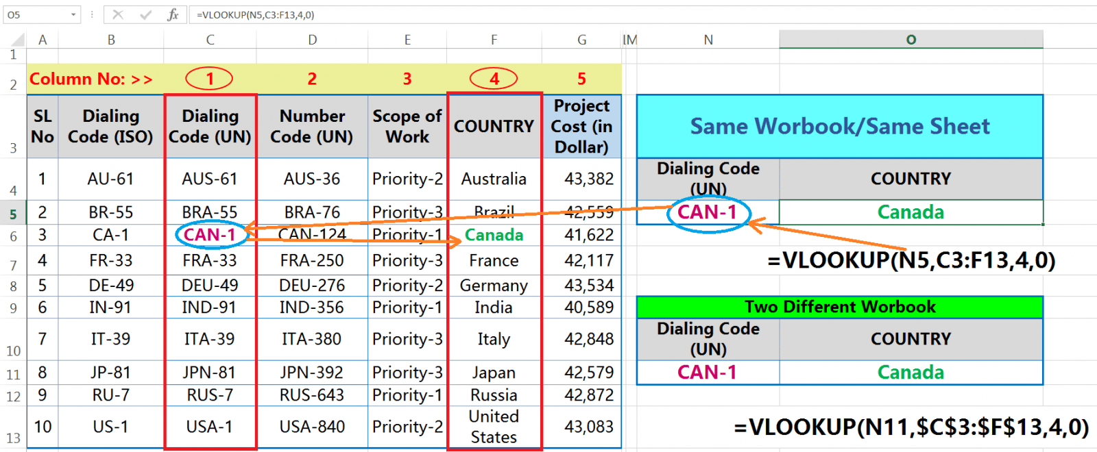
In the above example, if we want to retrieve the ‘COUNTRY’ name from column F, then the Excel VLOOKUP formula is written as =VLOOKUP(“CAN-1”, C3:F13, 4, 0). The formula searches the lookup_value “CAN-1” in the range of cells between C3 to C13 and returns a value from the range of cells between F3 to F13 in the same row. The count of columns between C and F is 4.
So, the column_index_number will be 4.
• range_lookup [Optional Argument]
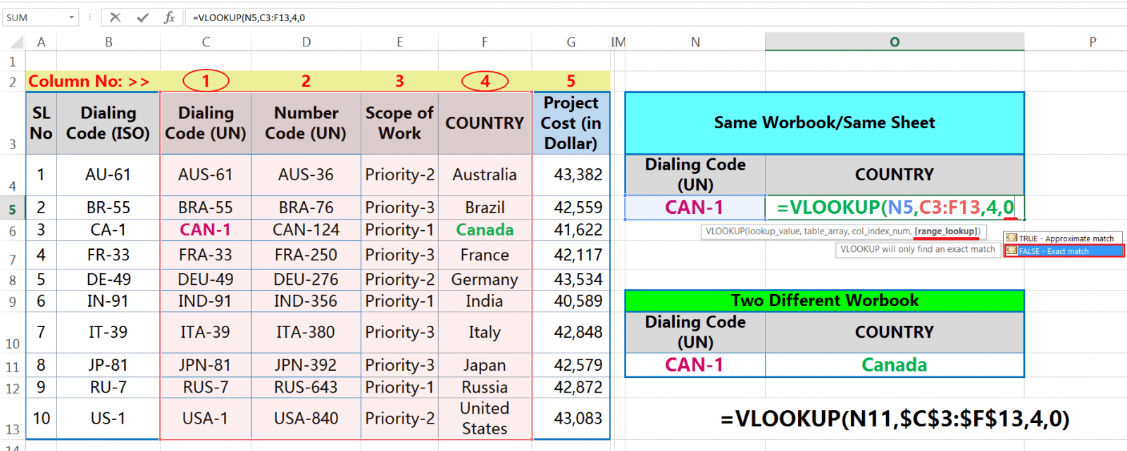
The range_lookup determines whether to search for an exact match (FALSE or numeric 0) or an approximate match (TRUE or Omitted or numeric 1). This is an optional argument, but very important.
- TRUE or 1 or omitted– the lookup function will return an approximate match. If an exact match is not found, the function will return the next largest value that is less than lookup_value. If the range_lookup is true, the first column of the VLOOKUP table must be sorted in ascending/alphabetical order; otherwise, the function will return the incorrect result.
- FALSE or 0 – the lookup function will return an exact match. IF the VLOOKUP function can’t find an exact match, the function returns the #N/A error. Remember that if the lookup_value is a text string, we can use wildcard characters (* and ?), but make sure that range_lookup is set to FALSE or 0.
In the above example, we are searching for the exact match, so the last argument in the Excel VLOOKUP formula will be either numeric zero (0) or FALSE. So the Excel VLOOKUP formula to be written as =VLOOKUP(“CAN-1”, C3:F13, 4, 0)
Finally, press Enter to accept the formula and Excel will close the last parenthesis by default if we do not close.
As a result, we get the result COUNTRY name ‘CANADA‘ against the lookup_value ‘CAN-1‘.
(C). EXCEL VLOOKUP EXAMPLE: FIND AN EXACT MATCH
Step to Start:

• When the lookup_value is a text: =VLOOKUP(“CAN-1“, C3:F13, 4, 0)
• To make the formula more dynamic by using the cell reference in place of the lookup_value: =VLOOKUP(N5, C3:F13, 4, 0)
➢ STEP 1: A PLACE (BLANK CELL) IS REQUIRED FOR THE EXCEL VLOOKUP FORMULA
Select the cell to get the result of the VLOOKUP function (i.e., the cell O5); generally, it is the blank place right to the lookup_value in the same row. In the given example, cell O5 is the blank place right to the lookup_value located in cell N5.
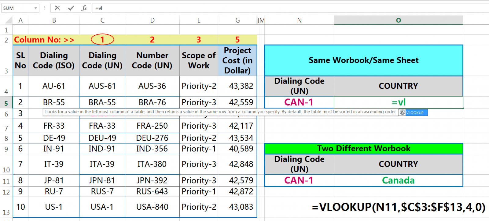
Select the cell O5, then press an equality ‘=‘ sign to start the formula and just type a few letters of the VLOOKUP function, such as =vlo….. Then select the VLOOKUP function from the below Excel provided auto-suggestion list with the help of a down arrow (↓), if required.

After selecting the VLOOKUP function, press the ‘Tab’ key. As a result, the VLOOKUP function syntax will appear with an open parenthesis.
Please note that the syntax in an upper or lower case does not matter, EXCEL by default considers it as an upper case.
➢ STEP 2: PLACING OF THE FIRST ARGUMENT LOOKUP_VALUE
We select a text or the cell reference in place of the lookup_value, the first argument of the Excel VLOOKUP function. It is also called the ‘field of the starting point‘.
In the given example, “CAN-1” is the text and is located in cell N5, which means the cell reference of “CAN-1” is N5. We can write the formula either in two ways:
(i) We can write as a text and to be written in a double quotation mark (” “) and place a comma (,) just after which indicates the closing of the first argument and command to move the next argument. For example, =VLOOKUP(“CAN-1“,
(ii) Otherwise, we can consider a cell reference and place a comma (,) just after which considers the closing of the first argument. Please keep in mind that any double quotation mark does not require in case of a numeric value or the cell reference. Moreover, we always try to consider the cell reference(s) in the argument(s), so the formula becomes more dynamic, which means any changes in the cell will affect the result of the formula. For example, =VLOOKUP(N5,
⇒ Note:
• We always prefer to use a dynamic Excel VLOOKUP formula rather than manual changing so that we do not require to change the formula every time after making any changes in the condition of lookup_value. Due to this reason, we always prefer to use a cell reference.
• Additionally, we make the Excel VLOOKUP formula more dynamic by fixing the cell references.
• The position of lookup_value may be the left, right, upward, and downward; but it doesn’t matter with the Excel VLOOKUP formula which means the formula works perfectly in any lookup position.
• We place a comma (,) after the completion of any argument in any formula which indicates that the placement of the current argument has been done; additionally command to Excel to move the next argument.
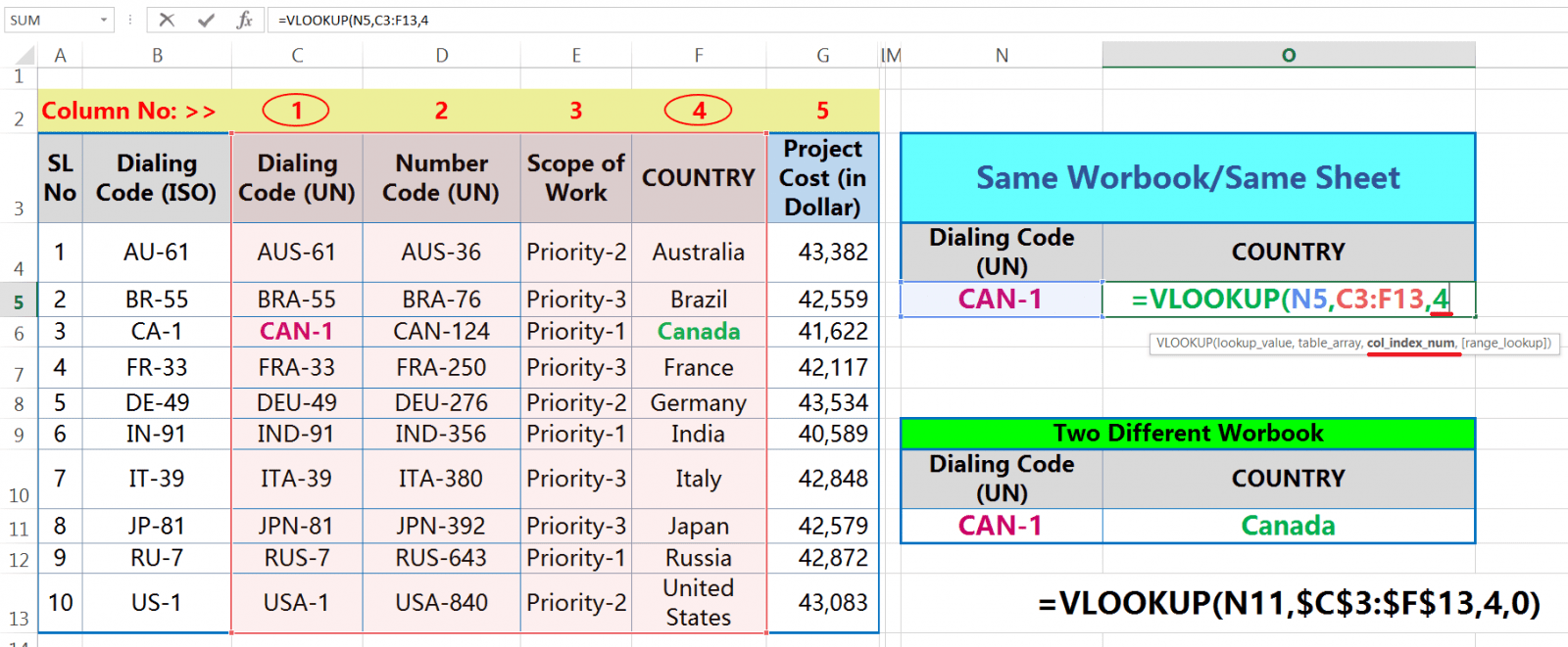
➢ STEP 3: PLACING THE SECOND ARGUMENT TABLE_ARRAY
The second argument of the Excel VLOOKUP function is the table_array, which is the range (one or more columns of data) that contains the lookup table from where the Excel VLOOKUP formula retrieves the data. It is also called the ‘information table‘.
The table_array can be located in the same (or existing) workbook or a different workbook.
A table_array should have a lookup column (i.e., the first column) and the result column (i.e., the column from where the value to be retrieved). The lookup column and the result column may be the same (when selecting the single column) or different.
In the given example, C3:F13 is a table_array, a rectangular grid of cells starting from cell C3 and ending in cell F13.
We would like to retrieve the data ‘COUNTRY’ name from the table_array in respect to the lookup value “CAN-1”. Where “CAN-1″ is found in the lookup column ‘C’ and ‘COUNTRY’ name is found in the result column ‘F’. So the range for the table_array will be C3:F13. Generally, we consider the Subject heading in the table array.
• C3 – table_array starts from column ‘C’ and row address is ‘3’ (first cell of the table).
• F13 – table_array ends in column ‘F’ and row address is ’13’ (last cell of the table).
So, we can write the formula either: =VLOOKUP(“CAN-1“, C3:F13,
Or, =VLOOKUP(N5, C3:F13,

⇒ Note:
(i) The position of the table_array is important, where the lookup column is always located to the left and it should be the first column of the table_array. Whereas the position of the result column is always located to the right from where the value(s) to be retrieved.
For example, “CAN-1” is the lookup_value located in the column ‘C‘. So the table_array starts from here. Whereas ‘COUNTRY’ name is the retrieved value and is located to the right side, i.e., in the column ‘F‘. Thus, the table_array will be the C3:F13.
(ii) The Excel VLOOKUP function doesn’t work at all if the lookup column (i.e., “CAN-1”) is located to the right and the result column to the left of the table_array.
Because only the Excel VLOOKUP function doesn’t perform the reverse lookup, it always looks right and it is the biggest limitation of this function. But along with other functions, the Excel VLOOKUP function makes a nested formula that performs reverse LOOKUP.
(iii) In the given example, why we didn’t consider the column ‘A‘ (i.e., Sl No) and column ‘B‘ (i.e., Dialing Code (ISO)) in the table_array because the lookup_value “CAN-1” is not present in both the columns.
(iv) After placing the table_array argument we put a comma (‘,’) which indicates that the placement of the current argument has been done and additionally command to Excel to move the next argument.
➢ STEP 4: PLACING THE THIRD ARGUMENT COL_INDEX_NUM
The third argument of the Excel VLOOKUP function is col_index_num. It considers the total count of columns between the lookup column and the result column in a table_array. It is always an integer/numerical value. In the given example, the total count of columns between C and F is 4. So, 4 is the column_index_number.
After selecting the range C3:F13, the formula shows the selected range denomination like 11R x 4C.
• 11R – 11 rows are selected in the table_array range. ‘R’ stands for ‘ROWS’. The count of rows plays an important role in the HLOOKUP function.
• 4C – 4 columns are selected in the table_array range. ‘C’ stands for ‘COLUMNS’. The count of columns is considered in the VLOOKUP function.
So we consider the col_index_number in the Excel VLOOKUP formula is 4 and we can write the formula as =VLOOKUP(“CAN-1”, C3:F13, 4
Or, =VLOOKUP(N5, C3:F13, 4
➢ STEP 5: PLACING THE LAST ARGUMENT RANGE_LOOKUP
The last argument of the Excel VLOOKUP function is the range_lookup. In most cases, the VLOOKUP formula is used for an exact match (FALSE or numerical 0), but it is also used for the approximate match (TRUE or numerical 1 or omitted).
If the lookup_value is a text string, then we always go for the exact match. In the given example, “CAN-1” is the lookup_value and it is the text. So we always try to search for an exact match i.e. FALSE or 0.
Thus, we can write the formula in 04 different ways:
=VLOOKUP(“CAN-1”, C3:F13, 4, 0)
Alternatively, =VLOOKUP(“CAN-1”, C3:F13, 4, FALSE)
=VLOOKUP(N5, C3:F13, 4, 0)
Alternatively, =VLOOKUP(N5, C3:F13, 4, FALSE)
➢ STEP 6: PRESS ENTER TO ACCEPT THE FORMULA
Finally, press Enter to accept the formula. Excel considers that all arguments in the formula are properly mentioned, the formula ends immediately and the last parenthesis closes by default, if not closed.
➢ STEP 7: TO FIX THE CELL REFERENCES IN THE FORMULA
If we want to copy the formula to other cells, then we should fix the cell references as per the dataset structure. In the given example:
(i) First, we select the lookup_value and press the F4 key thrice. As a result, the cell reference is converted to a mixed cell reference where the column being absolute but the row is relative. For example, $N5. If we copy the formula horizontally (row-wise), the column address remains fixed but the row number changes accordingly.
(ii) Secondly, select the table_array and press the F4 key once. As a result, the cell reference is converted to an absolute. For example, $C$3:$F$13. If we copy the formula horizontally (row-wise), the column address remains fixed but the row number changes accordingly.
■ Note: We had detail explained on Cell Reference in a separate tutorial. Request you read this tutorial: 03 Types of Excel Cell Reference: Relative, Absolute & Mixed
(D). EXCEL VLOOKUP EXAMPLE: FIND AN APPROXIMATE MATCH
Like an exact match, we can use the Excel VLOOKUP function to approximate match, i.e., the range_lookup should set to ‘TRUE‘ (the default setting) or omitted or numeric ‘1‘. Generally, the approximate match function is applied where the lookup value is in number format rather than text format.
• =VLOOKUP(G3, B3:D11, 3, 1) – numeric 1 is used in range_lookup to get the approximate match; we get the result A-.
• =VLOOKUP(G5, B3:D11, 3, TRUE) – TRUE can be used in range_lookup instead of numeric 1; we get the same result A-.
• =VLOOKUP(G7, B3:D11, 3) – range_lookup can be omitted, the Excel VLOOKUP function will allow a non-exact match; we get result A-.
Before applying an approximate match function, the first thing we need to sort the first column of the table_array in ascending order. This is very important because the formula will stop searching as soon as it finds the nearest match smaller than lookup_value. If the data does not sort in ascending order, we will get incorrect or unexpected results or the #N/A error.
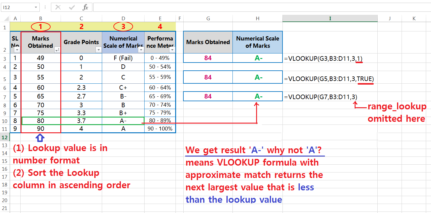
• WHY DO WE GET THE RESULT A- INSTEAD OF A?
Our lookup value is 84 and its closest values are 80 and 90 in the table. The formula returns A- rather than A, which means the VLOOKUP function retrieves the value against 80 instead of 90. Because the VLOOKUP formula with an approximate match retrieves the closest value that is less than the lookup value. The scale of marks against 80 is A-. Therefore, we get the result A- instead of A.
(E). EXCEL VLOOKUP EXAMPLE: FIND A PARTIAL MATCH (USING THE WILDCARD CHARACTERS)
We can use the following wildcard characters in the Excel VLOOKUP function for the partial match of lookup_value:
• Question mark (?) allows us to match any single character; and
• Asterisk sign (*) allows us to match any sequence of characters.
Wildcard characters are used in many cases:
(i) When we cannot remember the exact text looking for in the lookup_value.
(ii) When we want to find some word(s) or character(s) which are present in the cell’s contents.
• =VLOOKUP(‘CA*‘, C3:C12, 1, 0) – find the name starting with ‘CA’. The result is CAN-1.
• =VLOOKUP(‘*91′, C2:C12, 1, 0) – find the name ending with ’91’. The result is IND-91.
• =VLOOKUP(‘U*1′, C2:C12, 1, 0) – find the name starting with ‘U’ and ending with ‘1’. The result is USA-1.
• =VLOOKUP(‘?????‘, C2:C12, 1, 0) – find the 5-character name. The result is CAN-1. It is the first 5-character name in range C2:C12.
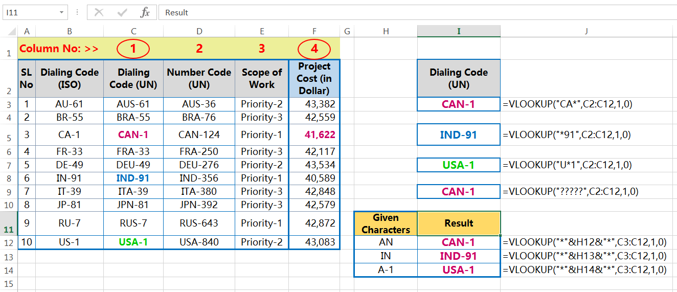
If we have only a few characters of the lookup_value, then we can get the result easily with the help of the VLOOKUP formula and the wildcard characters. Please notice that we use an ampersand (&) sign before and after a cell reference to concatenate a text string.
The position of characters may be in the middle, first or last it does not matter at all, place an asterisk symbol at the beginning and an asterisk symbol at the end and place the cell reference in between.
=VLOOKUP(“*“&H12&”*“‘, C2:C12, 1, 0)
We can get the desired result! Just follow the given figure.

(F). IMPORTANT FEATURES OF THE EXCEL VLOOKUP FUNCTION
➢ EXCEL VLOOKUP FUNCTION FEATURE 1: RIGHT LOOKUP
The Excel VLOOKUP function always looks for a value in the leftmost column of a table_array (lookup column) and returns the corresponding value from the right column (Result Column). This phenomenon of the Excel VLOOKUP function is called the right lookup.
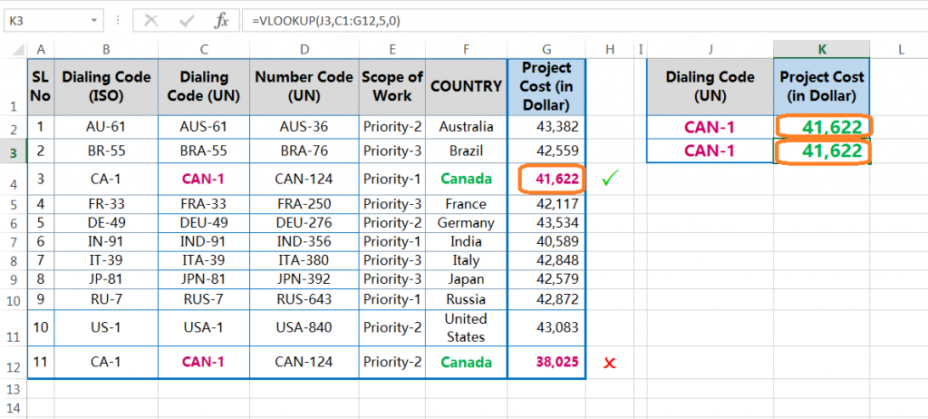
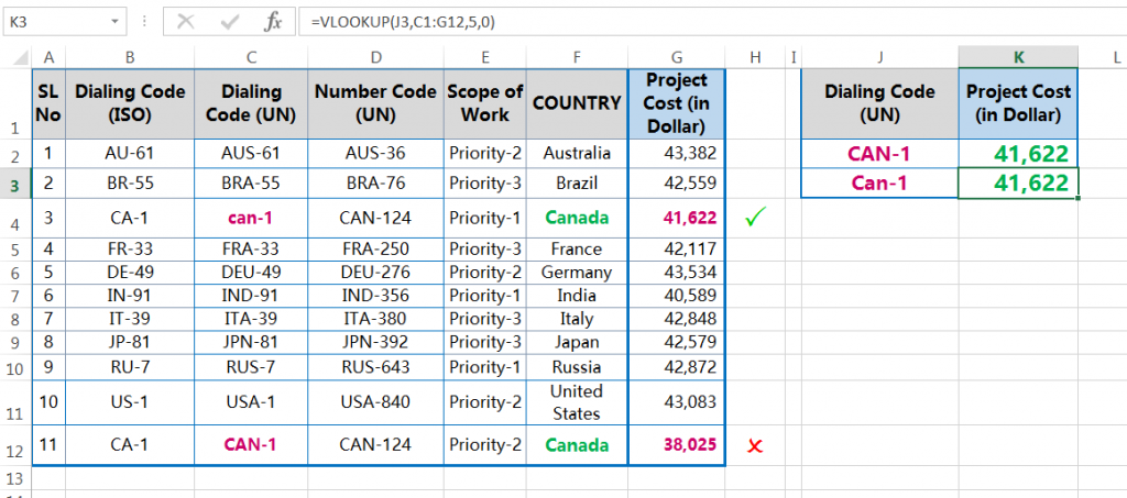
➢ EXCEL VLOOKUP FUNCTION FEATURE 2: FIRST MATCH
If the lookup_value (e.g., CAN-1) in the table array contains duplicates, the Excel VLOOKUP function match only the first instances. This phenomenon of the Excel VLOOKUP function is called the first match.
In the given example, CAN-1 has duplicated value in the table array. If we want to get the project cost of both the same instances, we only get the same value for both cases.
➢ EXCEL VLOOKUP FUNCTION FEATURE 3: CASE INSENSITIVE
The Excel VLOOKUP function is case insensitive, which means that the Uppercase and the Lowercase characters are treated as equivalent.
N.B.: INDEX, MATCH, and EXACT function altogether to perform a case-sensitive lookup.
➢ EXCEL VLOOKUP FEATURE 4: VLOOKUP FORMULA RETURNS #REF! ERROR & #N/A ERROR
➢ #REF! Error
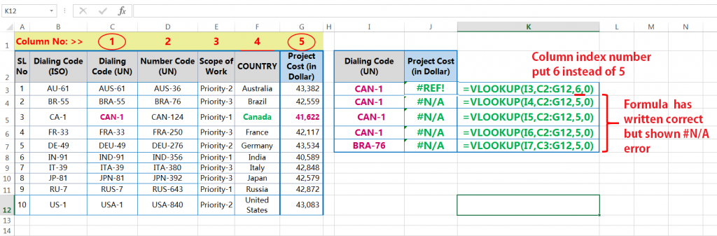
If we get a #REF! Error, first we recheck the formula and correct it. Generally, if we put the col_index_num more than the selected table_array, it returns a #REF! Error.
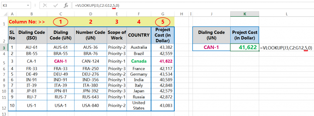
For example, we are selecting the table_array C2:G12 which means the count of columns in between the range is 5. So in this case, if we put column_index_num as 6 instead of 5 showing a #REF! Error.
➢ #N/A Error
If we get a #N/A Error, even the formula has written correct, then check the following parameters:
• If there is an extra space after the lookup_value, it returns a #N/A Error. For example, there is an extra space after ‘CAN-1’.

• If there is an extra space before the lookup_value, it returns a #N/A error.

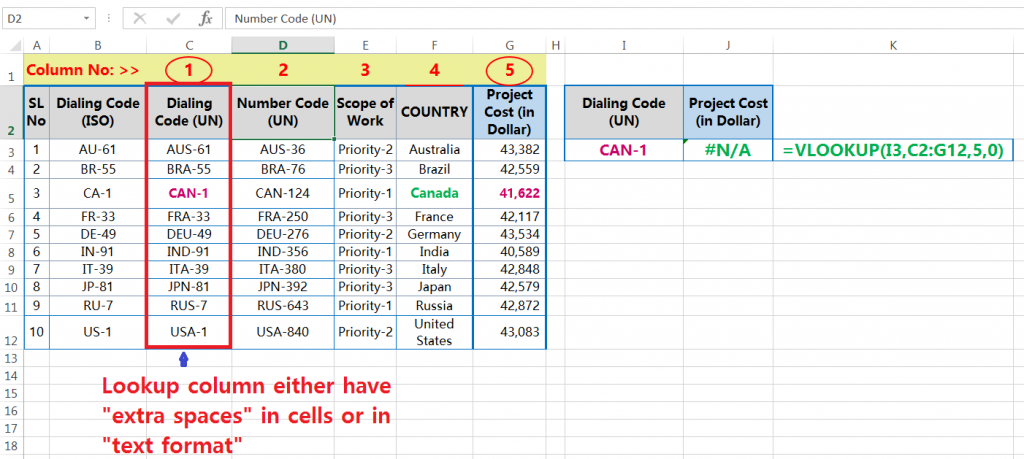
• If the lookup_value is in a text format, it returns a #N/A error. So, in that case, we should turn them into a general format.
• If the VLOOKUP function cannot find a match, it returns a #N/A error. This error can be modified with any kind of message or the formula by the IFERROR function.
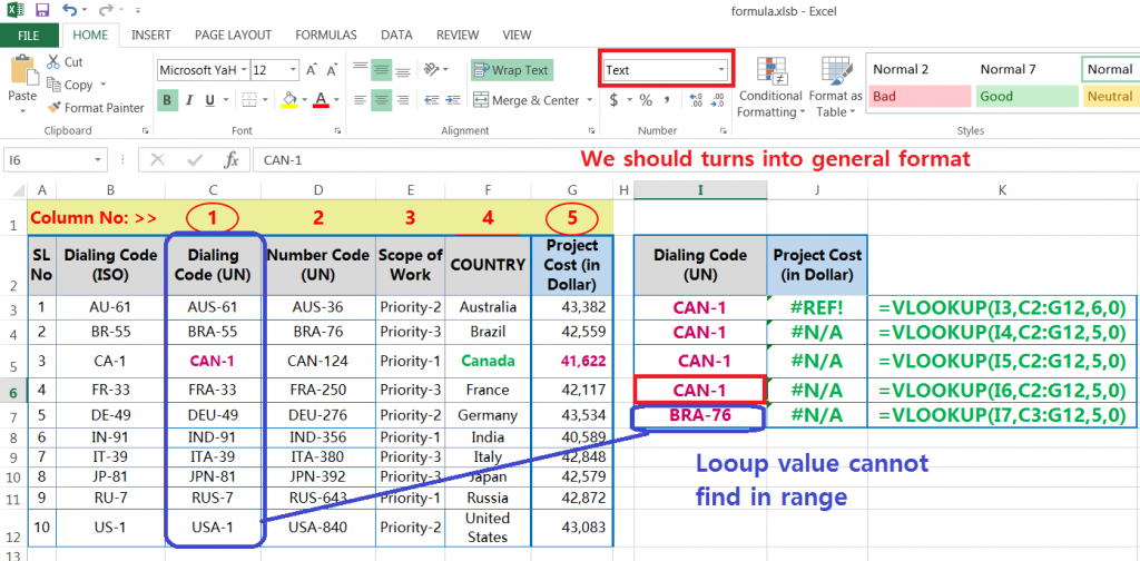
• Like lookup_value, if the lookup column is in text format, the VLOOKUP function also returns a #N/A Error. We need to convert the text format into the general format from any of the following 03 ways:
(a) by using the Convert Text to Column Wizard
(b) by using the Format Cells dialog box with the help of the excel shortcut Ctrl+1 ➪ Then select General.
■ Note: We had detail explained on the Ctrl Shortcuts in a separate tutorial. Request you read this tutorial: 90+ Best Excel CTRL Shortcuts | Useful Keyboard Shortcuts |
(c) by using the excel shortcut Alt+H+N (sequentially press Alt, H, N) and type General.
■ Note: We had detail explained on the Alt Shortcuts in a separate tutorial. Request you read this tutorial: 80+ Excel Shortcuts with ALT Key || Best Hotkey of Keyboard Shortcuts
• If there are extra spaces that exist in the lookup column, the Excel VLOOKUP function also returns the #N/A error. We should remove these extra spaces in two ways:
(a) by using the Convert Text to Column Wizard.
(b) by using the TRIM, SUBSTITUTE, and CHAR combined formula.
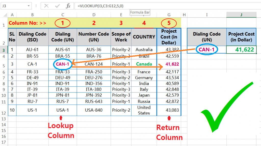
➢ EXCEL VLOOKUP FEATURE 5: VLOOKUP FORMULA BREAKS AFTER INSERTING/DELETING A COLUMN IN A TABLE ARRAY
The below figure showing the performance of a vlookup formula in Excel.
01. What will happen after inserting a column within the table_array?

After inserting a column anywhere in the table_array, the retrieved value is also changed. For example, a column inserts between Column ‘D’ & ‘E’ within the table_array, then the retrieved value shifted one column before.
However, after inserting a column (using Excel shortcut Ctrl++), col_index_num 5 now indicates the column ‘COUNTRY’ instead of ‘Project Cost (in Dollar)’. As a result, the VLOOKUP function retrieves the ‘COUNTRY’ name instead of ‘Project Cost (in Dollar)’.
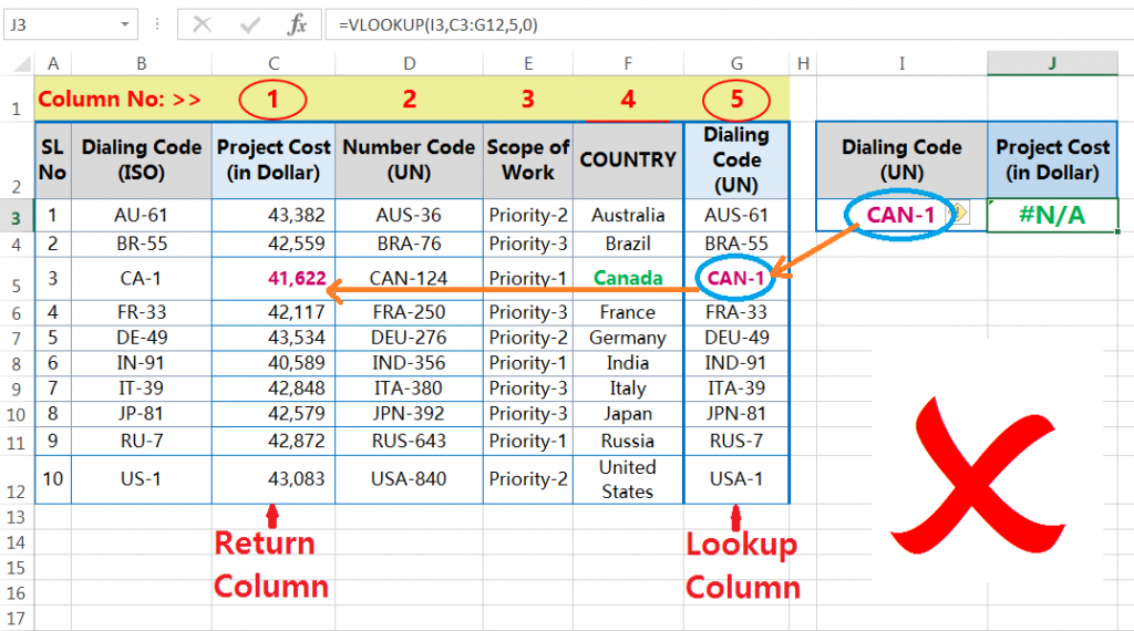
02. What will happen after deleting a column within the table_array?
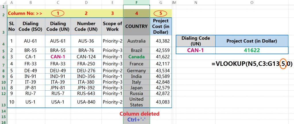
After deleting a column anywhere in the range (i.e., the table_array), the Excel VLOOKUP function returns a #REF! Error, because deleting a column, the range becomes smaller but the column number remains the same as before. So, in this scenario, the col_index_num will be more than the table_array.
For example, before deleting a column, the range was C3:G13 and col_index_num was 5. After the deletion of a column, the range becomes smaller C3:F13 and the col_index_num remain the same as 5 as before. But it should be 4 instead of 5. As a result, a #REF! Error returns. 
➢ EXCEL VLOOKUP FEATURE 6: VLOOKUP FORMULA WORKS WHILE REFERENCING TO ANOTHER WORKBOOK
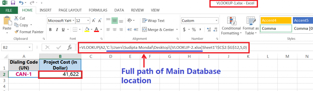
If the VLOOKUP formula refers to another workbook, once we close the workbook having a main dataset /table array, then the VLOOKUP formula works perfectly, but it displays the full path of the location of the reference workbook.

There are two workbooks. The lookup_value is placed in the workbook ‘VLOOKUP-1’ and the table_array (main database) is in the workbook ‘VLOOKUP-2’. The VLOOKUP formula in workbook ‘VLOOKUP-1’ refers to the workbook ‘VLOOKUP-2’. After closing the reference workbook ‘VLOOKUP-2’, we will find that the VLOOKUP formula works perfectly in the VLOOKUP-1 workbook, but it displays the full path of the location of that workbook.
Before Closing the VLOOKUP-2 Workbook:

After Closing the VLOOKUP-2 Workbook:
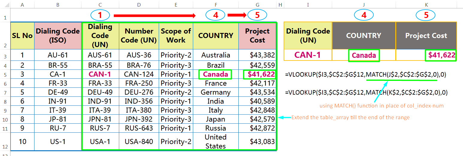
➢ EXCEL VLOOKUP FEATURE 7: EXTEND THE TABLE_ARRAY TILL THE END OF THE RANGE
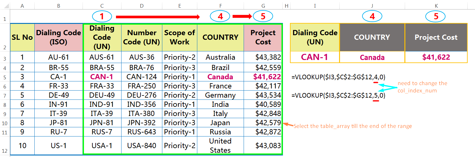
When we start working with the Excel VLOOKUP function, we must extend the table_array range till the end of the range. It is very much helpful to Lookup with the multiple columns or simply ‘Multiple VLOOKUP‘. In this case, we should change the col_index_number and get the result.
As a result, we do not require to apply the multiple times of VLOOKUP formula and manage time a lot for preparing the data analysis.
In the given example, extend the table_array till the end of the range. Put the number 4 as col_index_num to get the ‘Country’ name. After completing the VLOOKUP formula, fix the cell reference. Then copy (Ctrl+C) the formula to the right side. In this formula, change the col_index_num by 5 to get the ‘Project Cost’.
Equivalently, we use the MATCH() function in place of col_index_num which will make the dynamic formula. The MATCH function returns the relative position of a cell in a range that matches a specified value. So we don’t need to change the col_index_num manually.
(G). CONCLUSION
There is an important list of things to remember about the VLOOKUP function:
(01) The Excel VLOOKUP function always looks right and it is the biggest limitation of this function.
(02) If the lookup column contains duplicate values, The VLOOKUP formula will match the first value only.
(03) The Excel VLOOKUP function is case-insensitive, which means that uppercase and lowercase characters are treated as identical.
(04) The Excel VLOOKUP function is frequently used for exact matches (FALSE or zero ‘0‘) but it is less used for the non-exact or approximate matches (TRUE or omitted or ‘1‘).
(05) If the range_lookup is allowed for an exact match (FALSE or 0), then do not require to sort the lookup column of the table.
But if the range_lookup is allowed for an approximate match or non-exact match (TRUE or 1 or omitted), then the values in the lookup column (i.e., the first column) must be sorted in ascending / alphabetical order. Otherwise, the VLOOKUP formula returns an incorrect or unexpected value.
(06) The Excel VLOOKUP function with an approximate match retrieves the closest value that is less than the lookup value.
(07) If the lookup_value is a text string, we can use the wildcard characters (* and ?), but ensure that range_lookup is set to FALSE or 0.
(08) If there is an existing Excel VLOOKUP formula in the worksheet, in that case, the formula breaks even after inserting /deleting a single column in the table. This is so because the column index value (i.e., the col_index_num) doesn’t change automatically, even after the column(s) inserted/deleted.
(09) If the col_index_num is less than 1, the VLOOKUP formula returns a #VALUE! Error.
Similarly, if the col_index_num is greater than the number of columns in the table_array, the formula returns a #REF! Error.
(10) The VLOOKUP formula works in either the same workbook or another workbook. Once we close the reference workbook (having a table or dataset), then the Excel VLOOKUP formula works perfectly, but it will display the full path of the location of the reference workbook.
(11) Using a cell reference (dollar sign ‘$’) within the VLOOKUP formula makes the dynamic formula, which means the formula is copied to another location, cell references change automatically. Due to this, we do not require to apply the VLOOKUP formula multiply times.
(12) #N/A! Error – This error occurs while the Excel VLOOKUP function fails to find a match to the lookup_value.
(i) If there is an extra space after or before the lookup_value, it returns a #N/A error.
(ii) If the lookup_value is in text format, it returns a #N/A error. We should convert it into its general format.
(iii) If the first column (lookup column) of the table_array contains numbers entered as text, the formula returns #N/A! Error. Other than the first column in the table array may be in text format it does not matter, the Excel VLOOKUP formula retrieves data from the table.
(iv) If the Excel VLOOKUP function doesn’t find a match, it returns a #N/A error. This error can be replaced with any kind of message or formula with the help of the IFERROR function.
(13) #REF! Error – Occurs if either:
(i) The col_index_num argument is greater than the number of columns in the table_array, or
(ii) The formula is attempted to reference cells that do not exist.
(14) #VALUE! Error – Occurs if either:
(i) The col_index_num argument is less than 1, it does not recognize as a numeric value; or
(ii) The range_lookup argument is not recognized as one of the logical values TRUE or FALSE.
(15) The Excel VLOOKUP function allowing the use of a wildcard, i.e., an asterisk mark (*) or a question mark (?). While the asterisk mark is used for finding any number of characters, but each question mark is used for individual characters.
(i) =VLOOKUP(‘CA*‘,C3:C12,1,0) – find the name starting with ‘CA’. The result return: CAN-1.
(ii) =VLOOKUP(‘*91‘,C2:C12,1,0) – find the name ending with ’91’. The result return: IND-91.
(iii) =VLOOKUP(‘U*1‘,C2:C12,1,0) – find the name starting with ‘U’ and ending with ‘1’. The result return: USA-1.
(iv) =VLOOKUP(‘?????‘,C2:C12,1,0) – find the first 5-character name. The result return: CAN-1.
(16) Excel VLOOKUP function using fewer characters to give the name. Characters may be located in the first, middle or last of the name. For example,
(i) =VLOOKUP(‘*’&’AN‘&’*’,C3:C12,1,0) – find the name having ‘AN’. The result return: CAN-1. Characters are located in the middle.
(ii) =VLOOKUP(‘*’&’IN‘&’*’,C3:C12,1,0) – find the name having ‘IN’. The result return: IND-91. Characters are located in the first.
(iii) =VLOOKUP(‘*’&’A-1‘&’*’,C3:C12,1,0) – find the name having ‘A-1’. The result return: USA-1. Characters are located in the last.


Join Our Community List
Subscribe to our mailing list and get interesting stuff and updates to your email inbox.