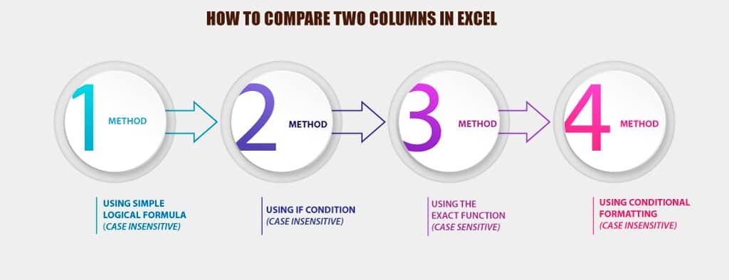
In this tutorial, we will explain How To Compare Two Columns In Excel (for differences and matches) and it is most important to identify the differences. Regularly, every Excel user tries to retrieve data from other files into the master file (usually with the help of the VLOOKUP function, INDEX MATCH function) and checks the latest update if any by any of the following 4 methods. However, users can update their master file with the changes (if any), so it helps to save a lot of time and reduces the gap of abnormality in the master file.   

(01) HOW TO COMPARE TWO COLUMNS IN EXCEL ➢ USING SIMPLE LOGICAL FORMULA (CASE INSENSITIVE)

We can create a simple logical formula to determine whether two cells contain the same entry. For example, use this formula to determine whether cell A2 has the same contents as cell C2:

=A2=C2

This formula will return either TRUE or FALSE, depending on the contents of cells A2 and C2.

However, Excel is a bit lax in its comparisons when text is involved. Consider the case in which A2 contains the word AUS-36 (all uppercase), and C2 contains aus-36 (all lowercase). We’ll find that the previous formula returns TRUE even though the contents of the two cells are not really the same. In other words, the comparison is not case-sensitive.

Step 1: At first, select cell D2, then place an equality sign (=) to start the formula. Then select the first cell A2, again place an equality sign (=) after A2, and select cell C2.

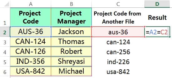
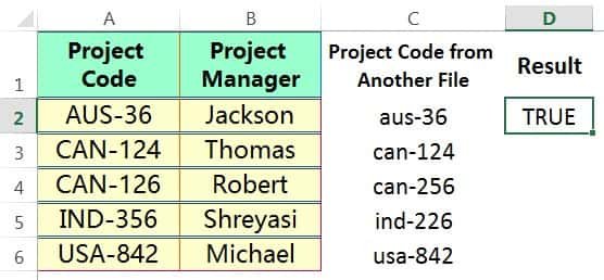
Step 2: Then simply press Enter or Ctrl+Enter, which will show either TRUE or FALSE. In this case, it will show TRUE which means the value in cell A2 is equal to the value in cell C2,  otherwise, it will show as FALSE.

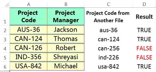
Step 3: Extend the formula downward till to the end of the range to get the results. 

● Read More: 06 Alternative Methods: How to Copy Formula in Excel?

(02) HOW TO COMPARE TWO COLUMNS IN EXCEL ➢ USING IF CONDITION (CASE INSENSITIVE)

If required, we can use the IF function to replace TRUE or FALSE with a specific text string. Please keep in mind that the IF formula returns the result based on criteria that may not be case-sensitive, which means criteria text may be upper, lower, proper case doesn’t matter at all. 

Before going to the formula, we will focus on the syntax for the IF function.

(01) We can use the IF function when we try to mention TRUE or FALSE. But in this case, we should mention them within double quotation (” “).

So the formula is written as:

=IF(A2=C2,”TRUE”,”FALSE”)

Then simply press Enter or Ctrl+Enter, which will show either TRUE or FALSE. In this case, it will show TRUE which means the value in cell A2 is equal to the value in cell C2,  otherwise, it will show as FALSE.

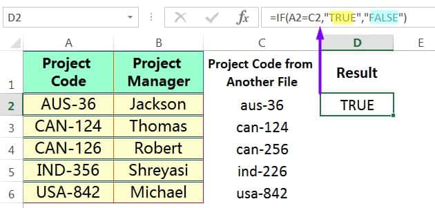
(02) We can use text strings in the IF function. Suppose, if the cell values between A2 and C2 are the same, the logic returns TRUE, then we can decide to replace it with the text “OK” and if the logic is FALSE then it replaces with the text “Not Matched“.

Thereafter the formula is written as:

=IF(A2=C2,”OK”,”Not Matched”)

Extend the formula downward till to the end of the range to get the results. 

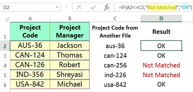
(03) We can arrange the logic in a different manner and based on the logic we should arrange the arguments respectively. Suppose, if the cell values between A2 and C2 are different, the logic returns TRUE, then we can decide to replace it with the text “Not Matched” and if the logic is FALSE then it is replaced with the text “OK“.

=IF(A2<>C2,”Not Matched”,”OK”)

(03) HOW TO COMPARE TWO COLUMNS IN EXCEL ➢ USING THE EXACT FUNCTION (CASE SENSITIVE)

Often, we don’t need to worry about the case of the text. If we need to make an exact, case-sensitive comparison, though, use the EXACT function.

The syntax for the Exact function is

(i) The function is case-sensitive and will return a TRUE or FALSE result. It is often used to compare two text strings to determine if they are the same, for example, the following formula returns TRUE only if cells A2 and C2 contain exactly the same entry: 

=EXACT(A2, C2)

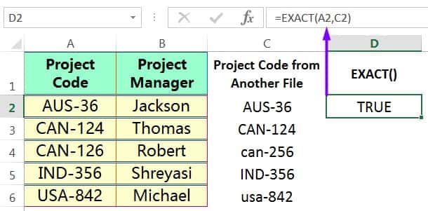
Then simply press Enter or Ctrl+Enter, which will show either TRUE or FALSE. In this case, it will show TRUE which means the value in cell A2 is equal to the value in cell C2, otherwise, it will show as FALSE.

Extend the formula downward till to the end of the range to get the results.

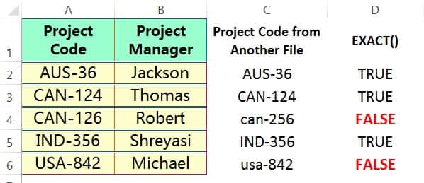
Note: When we compare text, be careful with trailing space characters, which are often difficult to identify. The following formula returns FALSE because the first string contains a trailing space:

=EXACT(“AUS-36  “,”AUS-36”)

When extra space is at the end of the text in a cell, it’s impossible to tell that it’s there just by looking at the cell. So if your text comparison formulas don’t seem to be working, a trailing space could be the problem.

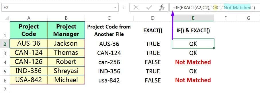
(ii) We can use text strings instead of TRUE and FAlSE with help of the IF function. Suppose, if the cell values between A2 and C2 are the same, the logic returns TRUE, then we can decide to replace it with the text “OK” and if the logic is FALSE then it replaces with the text “Not Matched“.

Thereafter the formula is written as:

=IF(EXACT(A2,C2),”OK”,”Not Matched”)

(04) HOW TO COMPARE TWO COLUMNS IN EXCEL ➢ USING CONDITIONAL FORMATTING (CASE INSENSITIVE)

We can highlight the rows that have matching data which means if the values of the cells meet a condition with similar values being highlighted. This returns case insensitive results which means both upper cases and lower cases are treated as identical.

(i) At first, select two columns from the entire dataset.

➢ If the columns are contiguous, press Ctrl+Spacebar which will select the single column, and then press Shift+Right arrow (➡) which will select the adjacent column to the right. 

➢ If the columns are non-contiguous, press Ctrl+Spacebar which will select the single column, then hold down the Ctrl key and click the column number which will select another column.

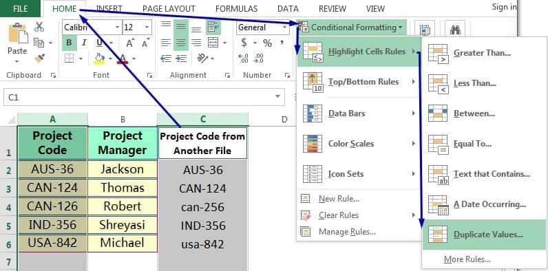
(ii) Go to the Home tab ➪ Click on the Conditional Formatting drop-down arrow in the Styles group ➪ Hover the cursor on the Highlight Cells Rules and as a result, a menu opens to the right ➪ Select the Duplicate Values…

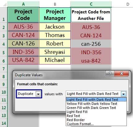
(iii) As a result, a Duplicate Values dialog box opens. By default, ‘Duplicate‘ is selected, and choose any formatting style from the values with drop-down list.

(iv) Finally, click OK or press Enter to accept the condition. 

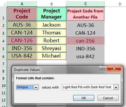
● Note: On the other hand, if we choose the Unique option it will highlight those cells containing unique values.