It is very essential in the Excel dashboard preparation that how to hide zero values in Excel? It gives the dashboard a unique appearance, easily visible the numbers, so anyone can analyze the data properly. 

In many of our daily worksheet calculations evaluate to zero, generally, we hide zero values. As a result, this will help to highlight those cells that contain actual numeric values and remove any distraction created by all the zeros.

Please remember that zero is considered a number and a blank cell has no numerical value. Hide zero values in excel is controlled on an individual worksheet, but other worksheets remain unaffected.

Method 1: Hide Zero Values in Excel by the ‘Workbook Settings’

The workbook settings will hide zeros in Excel. It is applicable for a particular worksheet, not for all the worksheets. 

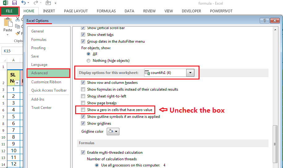
(01) Click on the ‘File’ menu at the corner.

(02) Click on ‘Options’ under it to open the Excel Options wizard.

(03) Choose the ‘Advanced’ from the sidebar menu.

(04) Scroll down to find ‘Display options for this worksheet’ and uncheck the box against “Show a zero in cells that have zero value”.

(05) Then click OK or press Enter.

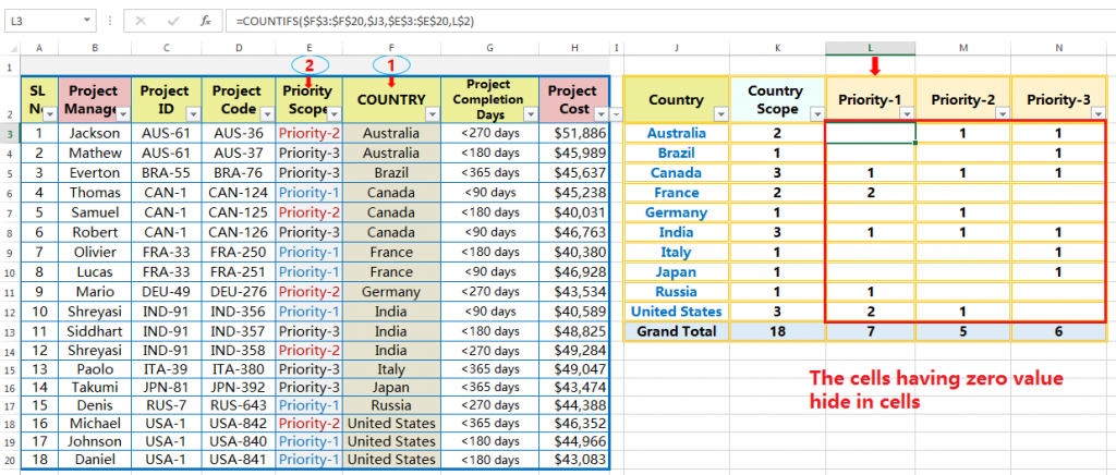
The zero values hide in cells, ranges, and the result as below as,

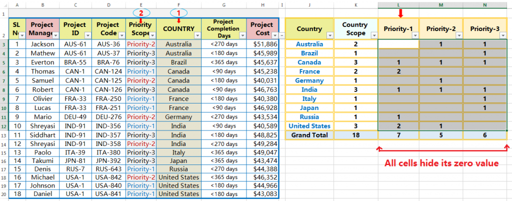
Please keep in mind that we can hide zeros in Excel in a particular worksheet, but not to all the worksheets. 

Method 2: Hide Zero Values in Excel by the ‘Format Cells’ Window

The ‘Format Cells’ window will allow us to hide specific zero values in Excel.

(01) Select the range of cells that contain zero values. For example, here the range is L3:N12.

(02) It is best practice to use the Excel shortcut Ctrl+1 to open the ‘Format cells’ Window ➪ Click on the ‘Number’ Tab.

A. Open ‘Format Cells’ using the Ribbon (via Number Section)

Click the Home tab ➪ then go to the Number section and click on Number settings (the small arrow in the bottom-right corner) that will open the Format cells wizard ➪ Click on the Number tab (if required).

Alternatively,

B. Open ‘Format Cells’ using the Ribbon (via Alignment Section)

Click the Home tab ➪ then go to the Alignment section and click on Alignment settings (the small arrow in the bottom-right corner) that will open the Format cells wizard ➪ Click on the Number tab.

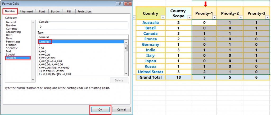
(03) Choose Custom from the Category list.

(04) Just type 0;-0;;@ in the Type field. Click OK or Enter.

As a result, hide zero values in Excel for a particular worksheet, not applicable to all the worksheets.

Note: If we want to undo this format, select General and click OK or press Enter.

Method 3: Hide Zero Values in Excel by the ‘Conditional Formatting Rules Manager’

The third method is conditional formatting allows us to hide zero values in a sheet. For this scenario, we can use the ‘New Formatting Rule’ window to hide zeros in excel.

Select the range of cells in which contain the zero values and want to hide. For example, here the range is L3:N12.

(01) We can open the ‘New Formatting Rule‘ window by 03 Methods:

A. Open ‘New Formatting Rule’ Window using the Excel Shortcut

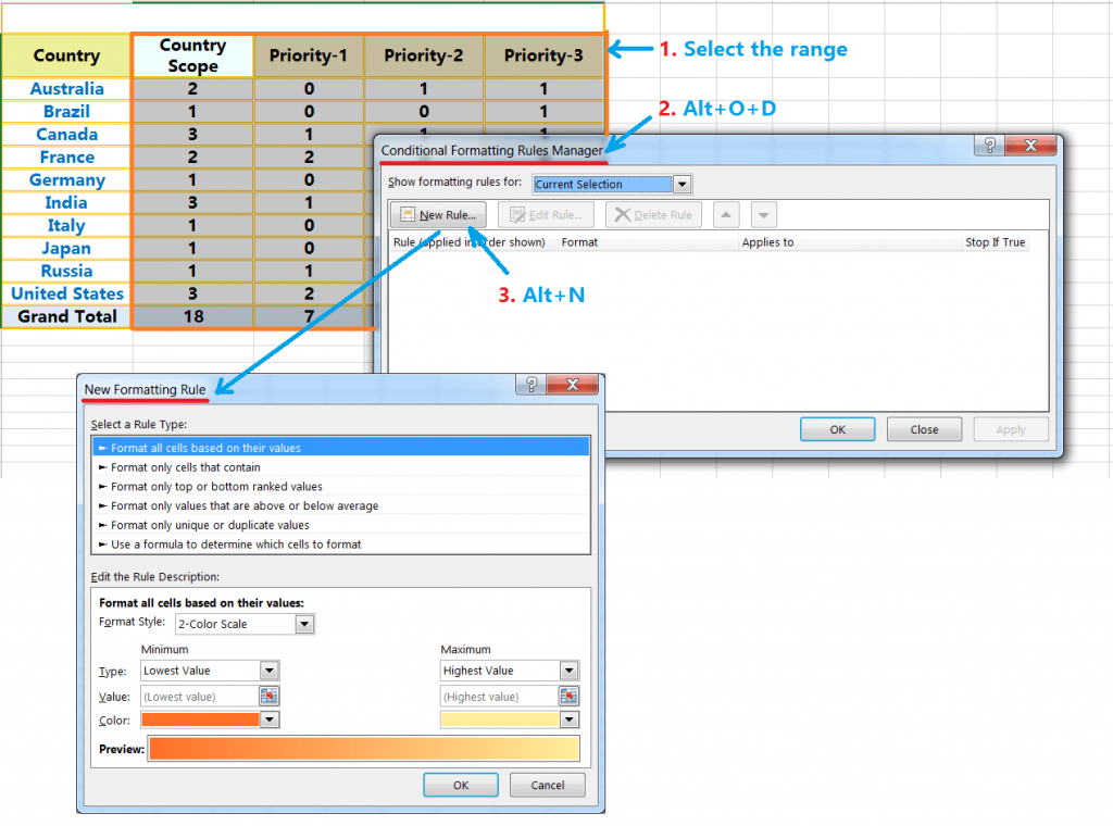
It is best to use the Excel shortcut by pressing Alt+O+D (press sequentially, Alt, O, D) o open the ‘Conditional Formatting Rules Manager‘ and then press Alt+N for New Rule or click on it ➪ As a  result, the ‘New Formatting Rule‘ window opens.

B. Open ‘New Formatting Rule’ using the Alternate Excel Shortcut

Press Alt+H+L+N (press sequentially, Alt, H, L, N) which will open the ‘New Formatting Rule‘ window.

C. Open ‘New Formatting Rule’ using the Ribbon

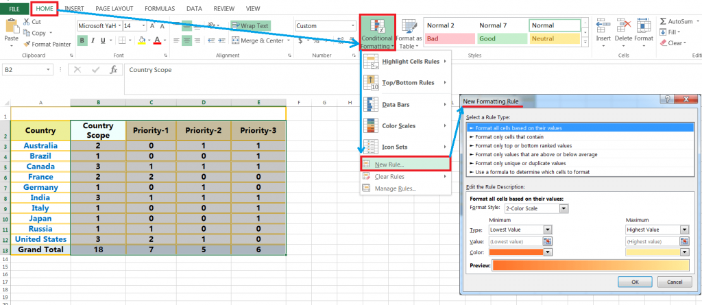
Click on the Home tab ➪ then click on the Conditional Formatting option in the Styles section ➪ Choose New Rule ➪ As a  result, the ‘New Formatting Rule‘ window opens.

(02) After opening the New Formatting Rule, select the second option ‘Format only cells that contain‘.

(03) From the second dropdown, choose ‘equal to‘.

(04) Enter zero (0) value in the third control.

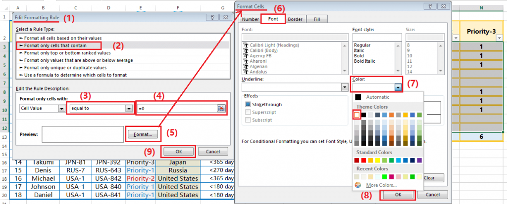
(05) Then click on the ‘Format’ box and open the ‘Format cells‘ window.

(06) Click on the Font tab.

(07) From the Color dropdown, choose the theme color White or choose the same color matching with the background. 

(08) Click OK which will close the ‘Format Cells’ dialog box.

(09) Again click OK which will close the ‘Edit Formatting Rule’ box.

Finally, we got the result. Remember that as a result hide zero values in Excel for a particular worksheet, not applicable to all the worksheets.