4 years ago 4 years ago

05 Points Should Learn How to Freeze Panes in Excel?

by Sudipta Mondal 4 years ago4 years ago

499views

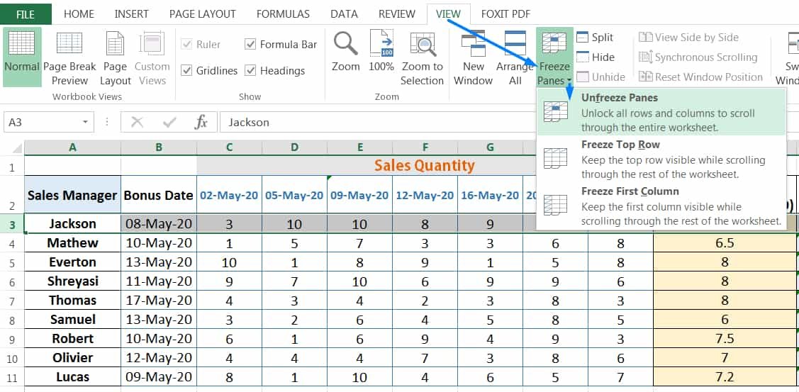
Freezing is the process of keeping rows and/or columns visible on screen at all times even when we scroll through a large dataset. When we apply freeze panes in excel, such as a row of column headings, the column headings remain visible as we scroll down the worksheet or change magnification.

So with the help of freeze panes in Excel, we can lock certain rows and columns at their place while we scroll throughout the worksheet. This is mostly required when we write a heading or a descriptive text in the first row or column and want it to stay in view while we fill up data against it.

04 Points Should Learn How to Freeze Panes in Excel

TABLE OF CONTENTS:

(01) EXCEL FREEZE PANES OPTIONS

Table: Freeze Options

Option	Description
Freeze panes	Keep both rows and columns above and to the left of the active cell visible as we scroll through a worksheet.
Freeze top row	Keeps only the top row visible as we scroll through a worksheet.
Freeze First Column	Keeps only the first column visible as we scroll through a worksheet.

(02) HOW TO FREEZE CELLS IN EXCEL?

or, HOW TO FREEZE COLUMNS AND ROWS IN EXCEL?

To freeze one or more rows and columns, use the Freeze Panes option. Before selecting this option, select an active cell one row below and one column to the right of the rows and columns we want to freeze.

■ Step 1: For example, to freeze the first two rows and the first two columns, we select a cell such as C3 and as a result, it becomes the active cell. ■ Step 2: Then we apply the Freeze Panes option either in two ways:

➢ Method 1 Apply Freeze Panes Shortcut:

After selecting the active cell, apply the Excel shortcut Alt+W+F+F (sequentially press Alt, W, F, F).

➢ Method 2 Apply Freeze Panes Using the Ribbon:

After selecting the active cell, Go to the View tab ➪ Click Freeze Panes drop-down ➪Select Freeze Panes. Thus, Excel displays a horizontal line below the last frozen row (row 2) and a vertical line to the right of the last frozen column (column B). Unfrozen rows (starting from row 3) and unfrozen columns (starting from C) are no longer visible when we scroll down and to the right, respectively. The frozen rows and columns are separated by dark lines. The frozen panes remain visible no matter how far we scroll away from the. If scrolled downwards, all the columns will scroll together, but the top row (containing the subject heading) will stay visible throughout. Likewise, when scrolled to the right, all the rows will scroll together, but the frozen column (the one containing the Bonus Date) will remain visible throughout.

(03) HOW TO FREEZE COLUMNS IN EXCEL?

➢ Method 1 Apply Freeze Panes Shortcut:

We can only freeze any column by selecting the very next adjacent column with Ctrl+Spacebar and then press Alt+W+F+F (sequentially press Alt, W, F, F). In the given example, we want to freeze column B. Thus, we select the very next adjacent column C with Ctrl+Spacebar ➪ then press Alt+W+F+F (press sequentially Alt, W, F, F).

➢ Method 2 Apply Freeze Panes Using the Ribbon:

We can select the column by clicking on the column address C at the top ➪ Then go to the View tab ➪ Click Freeze Panes drop-down ➪Select Freeze Panes. Note: If we have no specific choice to freeze panes in a specific column, then we apply Freeze First Column which will freeze the first column by default.

(04) HOW TO FREEZE A ROW IN EXCEL?

➢ Method 1 Apply Freeze Panes Shortcut:

We can only freeze any row by selecting the very next adjacent row with Shift+Spacebar and then press Alt+W+F+F (sequentially press Alt, W, F, F). In the given example, we want to freeze the 2ndrow with the subject heading. Thus, we select the very next adjacent row number 3 with Shift+Spacebar ➪ then press Alt+W+F+F (press sequentially Alt, W, F, F).

➢ Method 2 Apply Freeze Panes Using the Ribbon:

We can select the row by clicking on row number 3 on the left side ➪ Then go to the View tab ➪ Click Freeze Panes drop-down ➪ Select Freeze Panes. Note: If we have no specific choice to freeze panes in a specific row, then we apply Freeze Top Row which will freeze the first row by default.

(05) HOW TO UNFREEZE PANES IN EXCEL?

We can unfreeze the locked row and/or column either in 2 ways:

➢ Method 1 Using the Excel Shortcut:

Click any cell in the worksheet ➪ Then press Alt+W+F+F (sequentially press Alt, W, F, F).

➢ Method 2 Using the Ribbon:

Click any cell in the worksheet ➪ Go to the View tab ➪ Click Freeze Panes drop-down or arrow ➪ Select Unfreeze Panes.

If you would like to improve your academic and professional career as well, then the below courses help you a lot. Instead of Advanced Excel, a number of best courses suggested you through this platform that boosts your confidence and flies your career high.