TABLE OF CONTENTS:
ToggleWhat is a Filter in Excel?
The filter in Excel is a restriction that Excel uses to determine which rows to display from a range of data based on specified conditions or applied criteria and to display only those rows that meet those conditions/criteria. (After applying the filter, the other rows are hidden).
More technically, filtering is the process of specifying conditions for displaying records in a table or dataset. Only records that meet those conditions display; the other records are hidden.
We can use the filter on more than one column of a data range in Excel. Remember that, we can filter only by column, and not by row. In Excel, we have the ability to filter using various criteria such as date, value, text, and color.
After applying the filter in Excel, we can easily edit, copy, chart, or print only visible rows without rearranging the entire data set.
The items we see on the filter drop-down menu are called the filter criteria.
But the question arises in the mind that how to apply the filter in excel?
How to Filter in Excel?
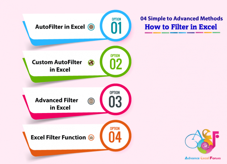
There are 5 methods to apply the filter in Excel:
(01) AutoFilter in Excel
(02) Custom AutoFilter in Excel
(03) Advanced Filter in Excel
(04) Excel Filter Function
■ METHOD 1: HOW TO USE AUTOFILTER IN EXCEL
The easiest way to filter an Excel database or table is to use Excel’s AutoFilter feature. An AutoFilter is the quickest tool to filter columns and set up a dataset/table so that it displays only rows that meet simple criteria.
➢ 06 Ways to Add AutoFilter in Excel
If a dataset/table with headings in the top row, it is the best practice to select the entire headings (by Shift+Spacebar) or to select the entire dataset (by Ctrl+A) ➪ then turn the Filter on/off feature using any of these methods:
• Method 1: Using Excel shortcut: Ctrl+Shift+L
• Method 2: Using Excel shortcut: Alt+A+T (sequentially press Alt, A, T)
• Method 3: Using Excel shortcut: Alt+D+F+F (sequentially press Alt, D, F, F)
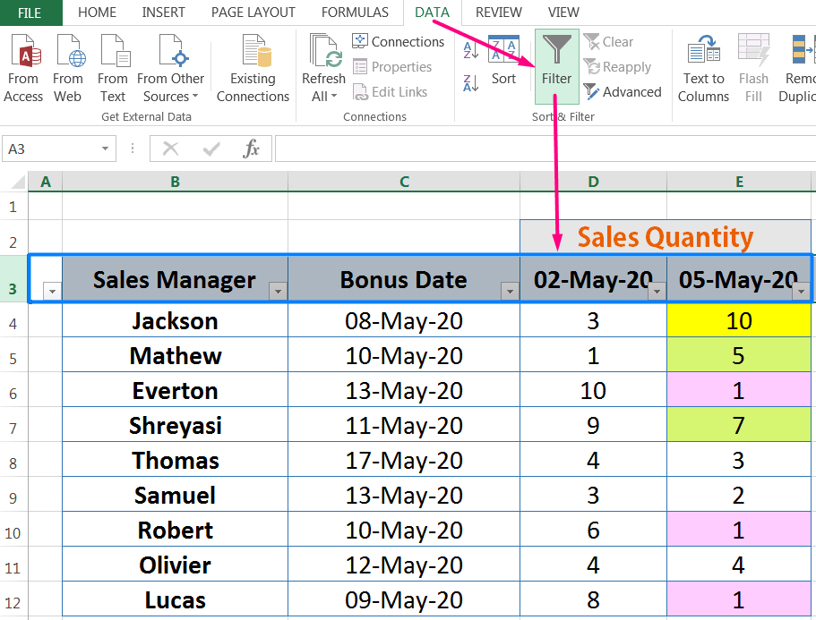
• Method 4: Using the Ribbon: Choose Data ➪ Filter from Sort & Filter section
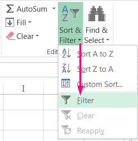
• Method 5: Using the Ribbon: Choose Home ➪ Sort & Filter ➪ Filter
• Method 6: Creating a Table from the dataset: Select the entire data set by Ctrl+A ➪ then press Ctrl+T.
By default, all new tables have their AutoFilter drop-downs turned on.

This step is optional. If we want to remove the alternate row bands from the table and make it a simple one, then we go to the Home tab ➪ Format as Table ➪ Choose Custom.

⇒ FAQ: Excel filter shortcut
➢ Excel Filter Options
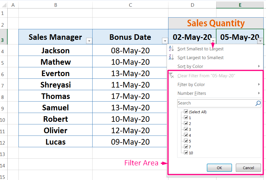
When we click the AutoFilter button, Excel recognizes the type of value (text, numeric, date) in the corresponding column and put the filter commands accordingly in the AutoFilter drop-down menu. The items we see in each drop-down menu are called the filter criteria.
(01) Text Filter
A text filter can find exact text, text that does not equal a condition, text that begins with a particular letter, and so forth.
When we apply a filter to a text field, the filter menu displays each unique text item. We can select one or multiple text items from the list to be filtered. Once completed only the selected text will be displayed.
➢ How to Apply Text Filter:
1. Before applying the Autofilter, it is the best practice to select the entire data set by pressing Ctrl+A or select the subject heading by pressing Shift+Spacebar.
2. Click the Data tab ➪ click Filter in the Sort & Filter group to display the filter arrows.
3. Click the filter drop-down for filtering a column ➪ Deselect the (Select All) checkmark.

4. Click the checkboxes for the text we would like to remain visible in the dataset ➪ Click OK.

➢ Example:
The above Figure shows the Sales_Manager filter menu with three names selected. Excel displays records for these three Sales Managers only. The records for the other sales managers are hidden but not deleted.
The filter drop-down displays a filter icon, indicating which field is filtered. Excel displays the row numbers in blue, indicating that we applied a filter. The missing row numbers indicate hidden rows of data. When we remove the filter, all the records display again.

➢ Text Filter Options:
We can also select Text Filters to see a submenu of additional options:
Table: Text Filter Options
Filter Option Description Equals Opens the Custom AutoFilter dialog box with the Equals operator selected in the first condition. Filters out the exact text/characters based on a specified text/characters. Does Not Equal Opens the Custom AutoFilter dialog box with the Does Not Equal operator selected in the first condition. Exclude the text/characters from filter based on a specified text/characters Begins With Opens the Custom AutoFilter dialog box with the Begins With operator selected in the first condition. Filters out the texts/characters begin with a specified text/characters Ends With Opens the Custom AutoFilter dialog box with the Ends With operator selected in the first condition. Filters out the texts/characters end with a specified text/characters Contains Opens the Custom AutoFilter dialog box with the Contains operator selected in the first condition. Filters out the texts/characters that contain a specified text/characters. Does Not Contain Opens the Custom AutoFilter dialog box with the Does Not Contain operator selected in the first condition. Filters out the texts/characters that do not contain a specified text/characters. Custom Filter Launches the Custom AutoFilter dialog box where we can specify our own criteria for more AND or OR conditions.
(02) Number Filter
A number filter can find exact values, values that do not equal a particular value; values greater than or equal to a value, and so on.
Excel contains a variety of number filters that enable us to display specific numbers or a range of numbers such as above average or top 10 values. When we filter a field of numbers, we can select specific numbers. Or, we might want to filter numbers by a range, such as numbers greater than 5 or numbers between 5 and 10.
➢ How to Apply Number Filter:
1. Select the entire data set by pressing Ctrl+A or select the subject heading by pressing Shift+Spacebar.
2. Click the Data tab ➪ click Filter in the Sort & Filter group to display the filter arrows.
3. Click the filter drop-down for filtering a column ➪ Deselect the (Select All) checkmark.
4. Click the checkboxes for the number we would like to remain visible in the dataset or we can enter a value in the Search box to display all matching records. For example, if we enter 5, the list will display only values that start with 5 (5, 50, 55, 525, 570 will be displayed) ➪ Click OK.

➢ Number Filter Options:
We can also select Text Filters to see a submenu of additional options:
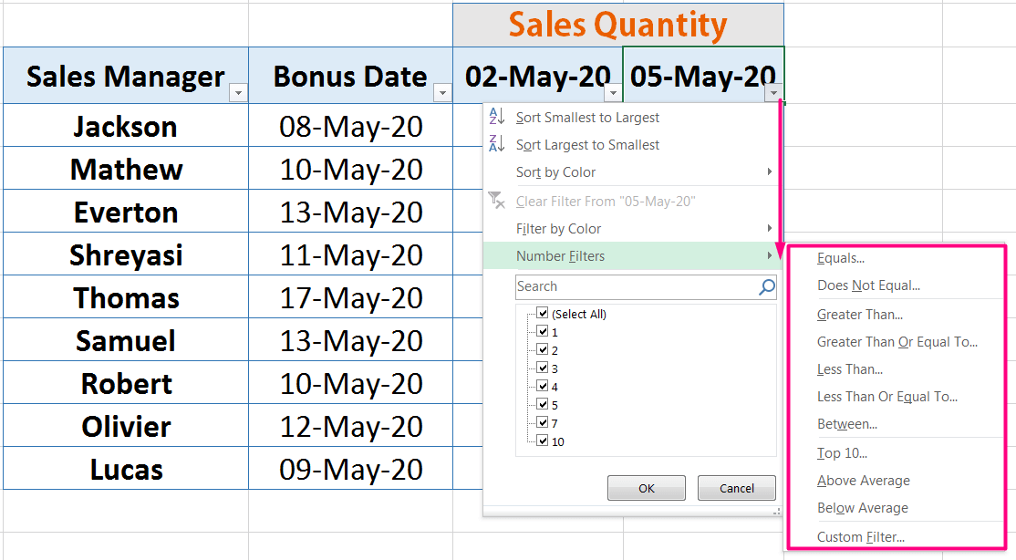
Table: Number Filter Options Filters out all the records, leaving behind the ones where the values in the selected field are greater than the average of the values in the same field. Filters out all the records, leaving behind the ones where the values in the selected field are less than the average of the values in the same field. Custom Filter Launches the Custom AutoFilter dialog box where we can specify our own criteria for more AND or OR conditions.Filter Option Description Equals Opens the Custom AutoFilter dialog box with the Equals operator selected in the first condition. Filters out the exact numbers/values based on a specified number/value Does Not Equal Opens the Custom AutoFilter dialog box with the Does Not Equal operator selected in the first condition. Exclude the numbers/values from filter based on a specified number/value Greater Than Opens the Custom AutoFilter dialog box with the Is Greater Than operator selected in the first condition. Filters out the numbers/values which are greater than the specified number/value Greater Than or Equal To Opens the Custom AutoFilter dialog box with the Is Greater Than or Equal To operator selected in the first condition. Filters out the numbers/values which are greater than or equal to the specified number/value Less Than Opens the Custom AutoFilter dialog box with the Is Less Than operator selected in the first condition. Filters out the numbers/values which are less than the specified number/value Less Than or Equal To Opens the Custom AutoFilter dialog box with the Is Less Than or Equal to operator selected in the first condition. Filters out the numbers/values which are less than or equal to the specified number/value Between Launches the Custom AutoFilter dialog box with the option Is Greater Than or Equal To selected in the first criteria and the Is Less Than or Equal To options selected in the second AND criteria. Top 10 Launches the Top 10 AutoFilter dialog box where we can specify the top 10 fields and filter out all leaving behind just the specified top 10 fields. Above Average Below Average
➢ Top 10 AutoFilter:
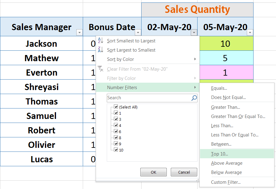
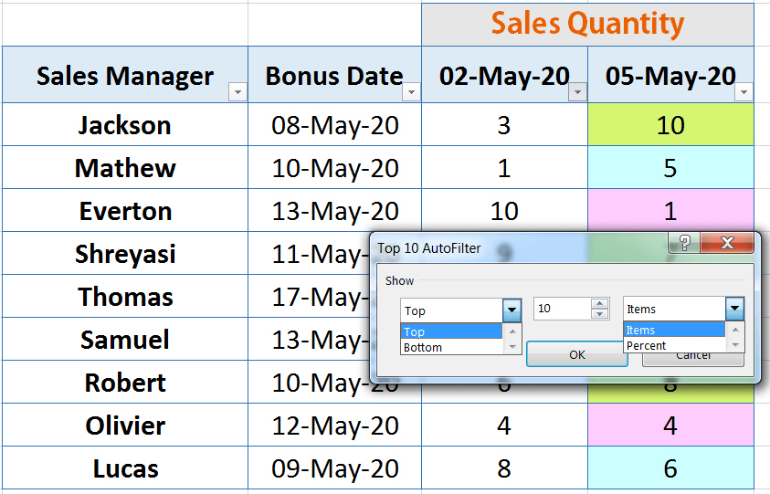
The Top 10 option enables us to specify the top records from a dataset/table. Although the option name is Top 10, we can specify the number (top or bottom “n” items) or percentage (“n%” of items) of records to display. For example, we can filter the list to display only the top 7 or the bottom 5%. The Figure shows below the Top 10 AutoFilter dialog box.
Steps to Start
(i) Select the entire range or table by Ctrl+A ➪ then press Ctrl+Shift+L or Alt+D+F+F (sequentially press Alt, D, F, F) which will apply the filter in the column’s header.
(ii) Click the filter drop-down for the column that contains the numeric data we would like to manipulate ➪ point to Number Filters ➪ select Top 10
(iii) Choose Top or Bottom value, click the last arrow to select either Items or Percent, and click OK or press Enter.
(03) Date Filter
A date filter can find dates before or after a certain date, between two dates, yesterday, next month, and so forth.
When we filter a field of dates, we can select specific dates or a date range, such as dates after 10-May-20 or dates between 10-May-20 and 20-May-20.
➢ Date Filter Options:
The submenu enables you to set a variety of date filters. For more specific date options, point to Date Filters, point to All Dates in the Period, and then select a period, such as Quarter 2 or May.

Table: Date Filter Options Next MonthFilter Option Description Equals Launches the Custom AutoFilter dialog box with the option equals selected in the first criteria. Filters out the exact dates from the dataset / table based on a specified date. Before Launches the Custom AutoFilter dialog box with the option is before selected in the first criteria. Filters out all the previous dates from the dataset / table based on a specified date. After Launches the Custom AutoFilter dialog box with the option is after selected in the first criteria. Filters out all the next dates from the dataset / table based on a specified date. Between Launches the Custom AutoFilter dialog box with the option is after or equal to selected in the first criteria and the is before or equal to options selected in the second AND criteria. Tomorrow Filters out all the records, leaving behind the ones with tomorrow’s date only. Today Filters out all the records, leaving behind the ones with the current date only. Yesterday Filters out all the records, leaving behind the ones with yesterday’s date only. Next Week Filters out all the records, leaving behind the ones with date entries in the week ahead. This Week Filters out all the records, leaving behind the ones with date entries in the current week. Last Week Filters out all the records, leaving behind the ones with date entries in the previous week. Filters out all the records, leaving behind the ones with date entries in the month ahead. This Month Filters out all the records, leaving behind the ones with date entries in the current month. Last Month Filters out all the records, leaving behind the ones with date entries in the previous month. Next Quarter Filters out all the records, leaving behind the ones with date entries in the 3-month quarterly period ahead. This Quarter Filters out all the records, leaving behind the ones with date entries in the current 3-month quarterly period. Last Quarter Filters out all the records, leaving behind the ones with date entries in the previous 3-month quarterly period. Next Year Filters out all the records, leaving behind the ones with date entries in the calendar year ahead. This Year Filters out all the records, leaving behind the ones with date entries in the current calendar year. Last Year Filters out all the records, leaving behind the ones with date entries in the previous calendar year. Year to Date Filters out all the records, leaving behind the ones with date entries in the current year up to the current date in this field. All Dates in the Period Filters out all the records, leaving behind the ones with date entries in the quarter (Quarter 1 through Quarter 4) or month (January through December) that you select from its submenu. Custom Filter Launches the Custom AutoFilter dialog box where we can specify our own criteria for more AND or OR conditions.
(04) Color Filter
If we have used cell color, font color, or icon set, we can use the Filter by Color fly-out menu to show records that have a certain color.
• Steps to Start:
Click the filter drop-down arrow in the column’s header cell, and point to Filter by Color ➪ Select the desired color want to display.
➢ Example 1: Filter by Font Color

➢ Example 2: Filter by Cell Color

➢ Example 3: Filter by Cell Icon
![]()
➢ How to Reapply Filter in Excel?
After making any changes (edit or delete data) in filtered cells, Excel AutoFilter does not update the data automatically to reflect the changes. So, in that case, we have to ‘Reapply’ the filter to get the result. First, we click any cell within the filtered dataset, and then apply any of the following 4 methods:
• Method 1: Using Excel shortcut: Alt+Ctrl+L
• Method 2: Using Excel shortcut: Alt+A+Y (sequentially press Alt, A, Y)
• Method 3: Using the Ribbon: Choose Data ➪ Reapply from the Sort & Filter group

• Method 4: Using the Ribbon: Choose Home ➪ Sort & Filter ➪ Reapply

➢ How to Clear Filter in Excel?
(01) To Clear All Filters and Display All Records in a Dataset
We can clear all the filters in 4 ways:
• Method 1: Using Excel shortcut: Alt+A+C (sequentially press Alt, A, C)
• Method 2: Using Excel shortcut: Alt+D+F+S (sequentially press Alt, D, F, S)
• Method 3: Using the Ribbon: Choose Data ➪ Clear from the Sort & Filter group
• Method 4: Using the Ribbon: Choose Home ➪ Sort & Filter ➪ Clear
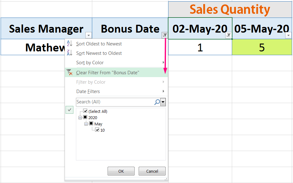
(02) To Clear One Filter in a Specific Column But Keep the Other Filters
If we want to clear only one filter in a certain column but keep the other filters, then we choose any one of the following methods:
• Method 1: Using Excel shortcut: First, select a filtered cell to want to clear filter ➪ Open the filter drop-down by pressing Alt+⬇ (Down arrow) ➪ then press Alt+C which will select Clear Filter From <“Column Heading Name”>.
• Method 2: Using Manual Way: Click the filter drop-down of a filtered cell to want to clear the filter ➪ then select Clear Filter From <“Column Heading Name”>.
➢ How to Remove Filter in Excel?
We can remove all the filters from the Excel worksheet in 5 ways. First, select a filtered cell or range of filtered cells then apply any of the following methods.
• Method 1: Using Excel shortcut: Ctrl+Shift+L
• Method 2: Using Excel shortcut: Alt+A+T (sequentially press Alt, A, T)
• Method 3: Using Excel shortcut: Alt+D+F+F (sequentially press Alt, D, F, F)
• Method 4: Using the Ribbon: Choose Data ➪ Filter from Sort & Filter section
• Method 5: Using the Ribbon: Choose Home ➪ Sort & Filter ➪ Filter
➢ How to SUM Filtered Data in Excel?
While the SUM function will total both visible and hidden rows, the SUBTOTAL function will exclude rows that are hidden in a filtered dataset.
The SUBTOTAL function calculates an aggregate value, such as SUM, COUNT, AVERAGE, MAX, MIN, etc., for displaying values in a range, table, or database.
The SUBTOTAL function is very useful when we have filtered a list of data to hide certain rows. Since SUBTOTAL only applies to visible rows, we can use it to create a dynamic total along with the filter. Simply add the SUBTOTAL function below the filtered list and include the entire list in the range. Then, when we apply different filters, the SUBTOTAL function will change depending upon which rows of data are visible.
The syntax for the SUBTOTAL Function is
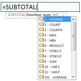
• The function_num argument is a number that represents a function (see below Table).
Table: SUBTOTAL Function Number for dataset and Table
| Function | Function number | Table number |
| AVERAGE | 1 | 101 |
| COUNT | 2 | 102 |
| COUNTA | 3 | 103 |
| MAX | 4 | 104 |
| MIN | 5 | 105 |
| PRODUCT | 6 | 106 |
| STDEV.S | 7 | 107 |
| STDEV.P | 8 | 108 |
| SUM | 9 | 109 |
| VAR.S | 10 | 110 |
| VAR.P | 11 | 111 |
• The ref1 argument indicates the range of values to calculate.
EXAMPLE:
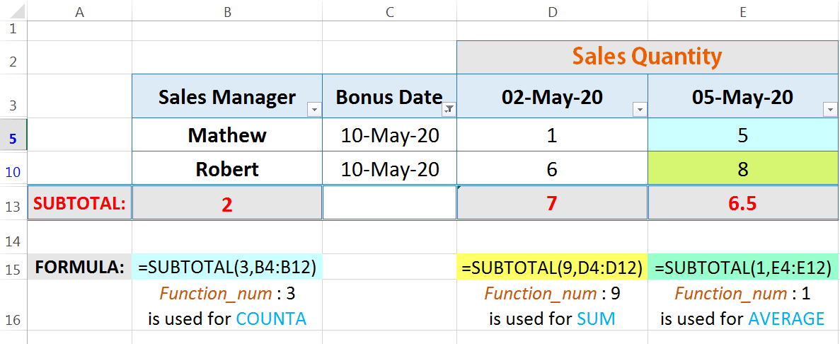
The figure provides below three examples of the SUBTOTAL function used with a filtered list.
(01) In cell B13, we use the formula =SUBTOTAL(3,B4:B12) for getting count value in the specified range B4:B12. Where the number 3 represents the COUNTA function,
(02) In cell D13, we use the formula =SUBTOTAL(9,D4:D12) for getting sum value in the specified range D4:D12. Where the number 9 represents the SUM function,
(03) In cell E13, we use the formula =SUBTOTAL(1,E4:E12) for getting the average value in the specified range E4:E12. Where the number 1 represents the AVERAGE function,

When the list is filtered, count, sum, and average values have been changed accordingly. A benefit of the SUBTOTAL function is that it subtotals data for filtered records, so we have an accurate total for the visible records.
For example, when we choose a particular bonus date (i.e., 10-May-20) from the filter dropdown, the SUBTOTAL function will show the total for that date.
• The COUNT value of the Sales Manager will be 2.
• The SUM value will be 7.
• The AVERAGE value will be 6.5.
➢ How to Copy Filtered Data in Excel?
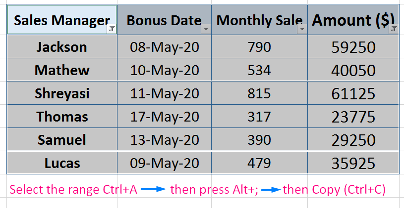
01. Select the entire filtered data range with Ctrl+A including column header.
Equivalently, select the first cell of filtered data ➪ then press Ctrl+Shift+➡ (right arrow) and Ctrl+Shift+⬇ (down arrow).
Equivalently, select the first cell of filtered data ➪ then press Ctrl+Shift+End
02. After selecting the range, press Alt+; to select only visible cells, thus we ignore hidden rows from coping.
Equivalently, Press Ctrl+G ➪ ‘Go To‘ dialog box ➪ Click ‘Special’ or press Alt+S ➪ ‘Go To Special‘ dialog box ➪ Select the radio button ‘Visible cells only‘ or press Alt+Y ➪ Click OK.
Equivalently, Press F5 ➪ ‘Go To‘ dialog box ➪ Click ‘Special’ or press Alt+S ➪ ‘Go To Special‘ dialog box ➪ Select the radio button ‘Visible cells only‘ or press Alt+Y ➪ Click OK.
03. Copy the filtered data by Ctrl+C.
04. Finally, go to the other location of the same worksheet or another worksheet or new workbook and do not press Ctrl+V to paste the filtered data, because if there are formulas in the filtered area it returns errors. So, in that case,
(i) Select a cell in the new location where to copy the range.
(ii) First, we press Alt+E+S+W (sequentially press Alt, E, S, W) or Alt+Ctrl+V+W (sequentially press Alt+Ctrl+V, W) which will select the ‘Column widths ‘ in the Paste Special dialog box. As a result, the copied data range arranges in a similar column width of source data.

(iii) If we want to copy formulas, then we apply Alt+E+S+R (sequentially press Alt, E, S, R) or Alt+Ctrl+V+R (sequentially press Alt+Ctrl+V, R) which will select the ‘Formulas and number formats‘ in the Paste Special dialog box. As a result, all the formulas and number formats are copied to the new location.

If we want to copy values instead of formulas, then we apply Alt+E+S+U (sequentially press Alt, E, S, U) or Alt+Ctrl+V+U (sequentially press Alt+Ctrl+V, U) which will select the ‘Values and number formats‘ in the Paste Special dialog box.
(iv) Thereafter, press Alt+E+S+T (sequentially press Alt, E, S, T) or Alt+Ctrl+V+T (sequentially press Alt+Ctrl+V, T) which will select the ‘Formats‘ in the Paste Special dialog box. As a result, the same source data formatting applied to the copied range.
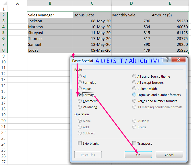
Finally, the copied range looks like

➢ How to Delete Filtered Data in Excel?
If we want to delete filtered data in Excel, then follow the below steps:
01. Select the first row just below the subject heading with Shift+Spacebar.
02. Then extend the selection downwards by pressing Ctrl+Shift+⬇.
03. After selecting the range, press Alt+; to select only visible cells, thus we ignore hidden rows from deleting.
04. Press Ctrl + – (minus) which will delete the selected rows.
■ METHOD 2: HOW TO USE THE CUSTOM AUTOFILTER IN EXCEL
A custom AutoFilter uses a rule that we create, instructing Excel how to evaluate the entries in each row and the basis of that evaluation determines which rows are filtered out.
We can use the Custom AutoFilter dialog box to configure the conditions. However, the conditions available in the Custom AutoFilter dialog box vary depending on the type of data in the column. We can set one or two conditions in the Custom AutoFilter dialog box.
We also specify the type of relationship between the two conditions with the ‘And’ or ‘Or’ option button. (The ‘And’ option button is selected by default.)
➢ Custom AutoFilter Options:
When selecting the operator for the first and second condition in the leftmost drop-down list boxes at the top and bottom of the Custom AutoFilter dialog box, we have the following choices, depending on the types of entries in the selected field:
| Filter Option | Description |
| Equals | Matches records where the entry in the field is identical to the text, date, or number we enter in the associated combo box. |
| Does Not Equal | Matches records where the entry in the field is anything other than the text, date, or number we enter in the associated combo box. |
| Is After | Matches records where the entry in the date field comes after the date we enter or select in the associated combo box. |
| Is After or Equal To | Matches records where the entry in the date field comes after or is the same as the date we enter or select in the associated combo box |
| Is Before | Matches records where the entry in the date field precedes the date we enter or select in the associated combo box. |
| Is Before or Equal To | Matches records where the entry in the date field precedes or is the same as the date we enter or select in the associated combo box. |
| Is Greater Than | Matches records where the entry in the field follows the text in the alphabet, comes after the date, or is larger than the number we enter in the associated combo box. |
| Is Greater Than or Equal To | Matches records where the entry in the field follows the text in the alphabet or is identical, the date comes after or is identical, or the number is larger than or equal to the one we enter in the associated combo box. |
| Is Less Than | Matches records where the entry in the field comes before the text in the alphabet comes before the date, or is less than the number we enter in the associated combo box. |
| Is Less Than or Equal To | Matches records where the entry in the field comes before the text in the alphabet or is identical, the date comes before or is identical, or the number is less than or equal to the one we enter in the associated combo box. |
| Begins With | Matches records where the entry in the field starts with the text, the part of the date, or the number we enter in the associated combo box. |
| Does Not Begin With | Matches records where the entry in the field starts with anything other than the text, the part of the date, or the number we enter in the associated combo box. |
| Ends With | Matches records where the entry in the field ends with the text, the part of the date, or the number we enter in the associated combo box. |
| Does Not End With | Matches records where the entry in the field ends with anything other than the text, the part of the date, or the number we enter in the associated combo box. |
| Contains | Matches records where the entry in the field contains the text, the part of the date, or the number we enter in the associated combo box. |
| Does Not Contain | Matches records where the entry in the field contains anything other than the text, the part of the date, or the number we enter in the associated combo box. |
➢ Filter column with One or Two Criteria:
There are basically 3 elements of the Custom AutoFilter dialog box.

(01) Filter Option drop-down menu:
To set the custom AutoFilter, click the first filter option drop-down arrows to select the comparison type, such as equals or contains. Click the drop-down arrow on the right to select a specific text, dates, or values, or type the data manually.
(02) And/Or Logical Operator Radio Button:
We can select the ‘And’ radio button whether both criteria should be true. (The ‘And’ option button is selected by default.)
We can select the ‘OR’ radio button whether a single criterion should be true.
(03) Parameter text fields/drop-down menu:
Define the specific criteria for the search and located right to the filter option drop-down menu. We can select a specific text, dates, or values, or type the data manually, which is populated with the column’s data entries.
• Example 1: Filter Numbers with Two Criteria
To create a filter that displays only Sales Amount between $400 and $800, a range of values so we select ‘And’ comparison operator in between the filter option.

Open the Filter drop-down by Alt+⬇ (down arrow) ➪ point to ‘Number Filters‘ ➪ Either choose an appropriate comparison operator from the list (in this example, we select Between…) or click ‘Custom Filter…‘ to create an own rule.
In the first filter option, select the option ‘is greater than or equal to‘ and type 400 (or select from the drop-down list if available) in the right side box.
Similarly, in the second filter option, select the option ‘is less than or equal to‘ and type 800 (or select from the drop-down list if available) in the right side box.
We select ‘And‘ logical operator in between the options ➪ finally click OK or press Enter.

• Example 2: Filter Dates with Two Criteria
To create a filter that displays only Bonus dates between 10-May-20 and 15-May-20, a range of dates so we select ‘And’ comparison operator in between the filter option.
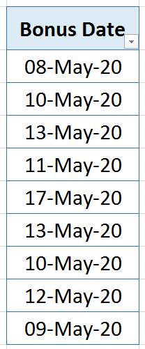
Open the Filter drop-down by Alt+⬇ (down arrow) ➪ point to ‘Date Filters‘ ➪ Either choose an appropriate comparison operator from the list (in this example, we select Between…) or click ‘Custom Filter…‘ to create an own rule.
In the first filter option, select the option ‘is after or equal to‘ and type 10-05-2020 (or select from the drop-down list if available) in the right side box.
Similarly, in the second filter option, select the option ‘is before or equal to‘ and type 15-05-2020 (or select from the drop-down list if available) in the right side box.
We select ‘And‘ logical operator in between the options ➪ finally click OK or press Enter.

• Example 3: Filter Texts with One or Two Criteria
• EXAMPLE WITH O CRITERION:
We create a filter that does not display a particular text string from the filtered list.

Open the Filter drop-down by Alt+⬇ (down arrow) ➪ point to ‘Text Filters‘ ➪ Either choose an appropriate comparison operator from the list (in this example, we select does not contain…) or click ‘Custom Filter…‘ to create an own rule.
Select ‘does not contain‘ in the first filter option and type ‘Thomas’ (or select from the drop-down list) in the right side box ➪ click OK or press Enter.
As a result, Sales Manager Thomas does not display in the filtered list.

• EXAMPLE WITH TWO CRITERIA:
If we want to filter two names from the filtered list, simply follow the few steps:
Open the Filter drop-down by Alt+⬇ (down arrow) ➪ point to ‘Text Filters‘ ➪ Either choose an appropriate comparison operator from the list (in this example, we select Between…) or click ‘Custom Filter…‘ to create an own rule.
In the first filter option, select the option ‘contains‘ and type Lucas (or select from the drop-down list if available) in the right side box.
Similarly, in the second filter option, select the option ‘contains‘ and type Shreyasi (or select from the drop-down list if available) in the right side box.
We select the ‘OR‘ logical operator in between the options ➪ then click OK or press Enter.

• Example 4: Filter Texts with Wildcard Characters
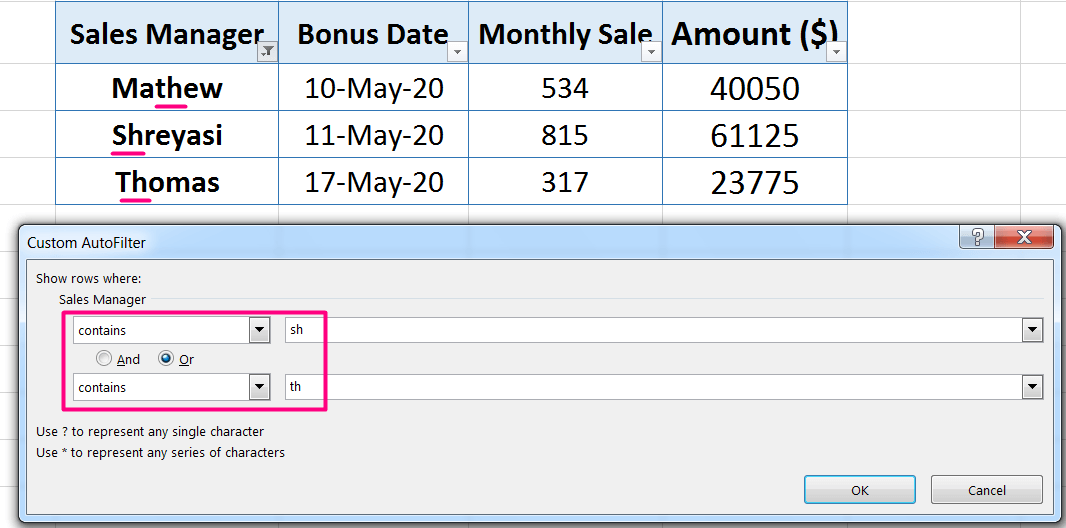
When filtering, if we don’t remember the exact search or want to filter out similar information, we can create a custom AutoFilter rule with wildcard characters. In these cases, we select the ‘Equal’ operator in the Filter Option and type the text chapters within the wildcard characters (e.g., *sh*, *th*, *s?*, *t?*, etc) in the right box. It helps out filter the desired text.
Note: We get the same result if we select the ‘Contains’ operator in the Filter Option and type the text (e.g., sh, th, s, t, etc) in the right box.
Steps to Start:
➢ Opening of Custom Filter: Open the Filter drop-down by Alt+⬇ (down arrow) ➪ point to ‘Text Filters‘ ➪ click ‘Custom Filter…‘. As a result, the Custom AutoFilter dialog box opens.

➢ Using Asterisk (*) Wildcard Characters: Asterisk (*) wildcard character matches any sequence of characters. For example,
(i) S* finds any length of text starting with S, e.g., Shreyasi, Samuel, etc.
(ii) *S finds any length of text ending with S, e.g., Thomas, Aurius, etc.
(iii) *S* finds any length of text contains S, e.g, Ostra, Sasha, Shreyasi, Samuel, Thomas, Aurius, etc.
In the below figure, we find out text with character sh and th from the Sales manager list.

Note: As mentioned above, we get the same result without wildcard characters if we choose contains in the filter option.
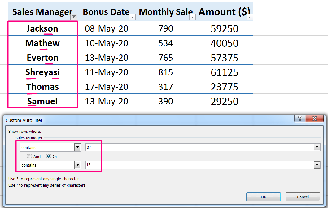
➢ Using Question Mark (?) Wildcard Characters: Question Mark (?) wildcard character matches any single character. For example,
(i) S? finds a single character after S, e.g., Sh, Sa, si, etc.
(ii) ?S finds a single character before S, e.g., as, us, etc.
(iii) ?S? finds a single character before S and a single character after S, e.g, Ost, ash, asi, etc.
In the below figure, we find out text with character sh and th from the Sales manager list.

Note: As mentioned above, we get the same result without wildcard characters if we choose contains in the filter option.
➢ Using Tilde (~) Wildcard Characters: Tilde (~) wildcard character is followed by *, ?, or ~. It allows filtering texts that really contain an asterisk (*), question mark (?), or tilde (~). Example as follows:

Example 1: Filtering out Asterisk (*) from a text string

• Alternative Method:

➢ Example 2: Filtering out Question Mark (?) from a Text String

• Alternative Method:

■ METHOD 3: HOW TO USE THE ADVANCED FILTER IN EXCEL
(01) Steps of Advanced Filter in Excel
➢ Define a Criteria Range
Before we apply advanced filtering, we must define the criteria range that is separate from the table or list, contains column labels, and lists the conditions on the row(s) immediately below the column labels in the criteria range. The conditions listed in the same row form an AND condition. Conditions on multiple rows form an OR condition.
A criteria range is a group of two or more adjacent cells that specifies the conditions used to control the results of a filter. The criteria row is often located below the dataset. A criteria range must contain at least two rows and one column. The first row contains the column labels as they appear in the dataset, and the second row contains the conditions (e.g., values) for filtering the dataset.
We can use <, >, <=, >=, =, and <> comparison operators, similar to using relational operators in the logical_test argument of an IF function. Using equal (=) and unequal (<>) symbols with the criteria values selects records with empty and nonempty fields, respectively.
Here are the requirements for creating a valid criteria range:
• The criteria range must contain the same column headings as the columns in the dataset/table. Column headings should be unique; try to avoid duplicate headings.
Note: The only problem with copying the field names to the criteria range is that if we change a field name, we must change it in two places—in the table/dataset and in the criteria range. So, instead of just copying the names, we can make the field names in the criteria range dynamic by using cell reference (place equality sign in a cell and set each criteria field name equal to its corresponding table field name). For example, we can enter =B2 in cell H2, =C2 in cell I2 so on.
• We cannot use cell or range references to define advanced filter criteria. We must manually enter values in the criteria range.
• Be aware that there may be some occasions where we do not need to enter an equal sign ( = ) operator. Simply enter the criteria may constitute that criteria equal to what we are looking to find.
• Criteria entered into cells on the same row in the criteria range use the AND operator. In other words, rows displayed in the filtered dataset must meet all of the specified criteria in the criteria range row.
• Criteria entered in different rows use the OR operator.
• Each criterion that we wish to include by using the OR operator must be in its own row in the criteria range.
• We can enter more than one filter operator in the same column. Not all columns have to include a filter operator.
• There must be no blank rows within the dataset we wish to filter.
➢ Comparison Operators
To define the criteria for advanced filtering, we use comparison operators. Comparison operators help us narrow search for specific data, and we can use these in nearly any combination.
Table: The Comparison Operators in the Selection Criteria
| Operator | Meaning | Description | Example |
| = | Equal to | Filter data based on an exact content match. As Excel interprets the equal sign as the beginning of a formula or function, you must enclose the = operator in a set of double quotation marks (” “). So, if we want to filter for all entries that include the text “IND”, we must enter the filter criteria as =”IND”. To filter for an exact numeric match, we can simply enter the numerical value. | (01) =”s” ➪ Records that contain the text begins with the letter S. For example, Shreyasi, Samuel, Sandrea, etc. (02) =”*s*” ➪ Records that contain the text includes the letter S. For example, Jackson, Shreyasi, Samuel, Lucas, etc. (03) =”s*” ➪ Records that contain text that includes letter S but does not end with S. For example, Jackson, Shreyasi, Samuel, etc. But it excludes Lucas. (04) =”*s” ➪ Records that contain text that ends with the letter S. For example, Lucas. (05) =”s*i” ➪ Records that contain text that begins with S and the letter i contains in the text. For example, Shreysi, Simon, Shine. |
| > | Greater than | Filters for numeric or date and time values that are greater than the defined criteria. | (01) >s ➪ Records that contain text that begins with a letter S and after S (that is, S through Z) (02) >5 ➪ Records the values which are greater than 5 (that is 6 or above 6) (03) >10/06/2020 ➪ Records the dates after June 10, 2020 |
| >= | Greater than or equal to | Filters for numeric or date and time values that are greater than or equal to the defined criteria. | (01) >=5 ➪ Records the values which are greater than or equal to 5 (that is 5 or above 5) (02) >= 10/06/2020 ➪ Records where the date is on or after or equal to June 10, 2020 |
| < | Less than | Filters for numeric or date and time values that are less than the defined criteria. | (01) ➪ Records where the name begins with a letter before E (that is, A, B, C, or D) (02) <5 ➪ Records the values which are less than 5 (that is 4 or below 4) (03) <10/06/2020 ➪ Records the dates before June 10, 2020 |
| <= | Less than or equal to | Filters for numeric or date and time values that are less than or equal to the defined criteria. | (01) <=5 ➪ Records the values which are greater than or equal to 5 (that is 5 or above 5) (02) <= 10/06/2020 ➪ Records where the date is on or before or equal to June 10, 2020 |
| <> | Not equal to | Filters for numerical, textual, or date and time values that are not equal to the defined criteria. | (01) <>”s” ➪ Records that text that does not contain the letter S. |
Table: The Wildcard Characters
| Operator | Meaning | Description | Example |
| * | Asterisk | An asterisk (*) matches any number of characters | (01) =”*s*” ➪ Records that contain the text includes the letter S. For example, Jackson, Shreyasi, Samuel, Lucas, etc. (02) =”s*” ➪ Records that contain text that includes letter S but does not end with S. For example, Jackson, Shreyasi, Samuel, etc. But it excludes Lucas. (03) =”*s” ➪ Records that contain text that ends with the letter S. For example, Lucas. (04) =”s*i” ➪ Records that contain text that begins with S and the letter i contains in the text. For example, Shreysi, Simon, Shine |
| ? | Question Mark | A question mark (?) matches any single character. | (01) m?r ➪ Records that contain March, Mario, Murli. (02) =”=?????” ➪ Records that contain exactly five letters (02) <>????? ➪ All records that do not contain exactly five letters. |
| ~ | Tilde | ~ (tilde) is followed by records that contain a real asterisk (*), question mark (?), or tilde (~). | (01) *~? ➪ Records that contain a single question mark character. (The tilde character overrides the wildcard question mark character.) For example, ?Stress, Stress?, Str?ess, ?Stress?. (02) *~* ➪ Records that contain any asterisk character. For example, *New Year, New*Year, New Year*, *New Year*. (03) ~* ➪ Records that begin with an asterisk character. For example, *New Year, *New Year*. (04) *~~ ➪ Records that contain any asterisk character. For example, *Birthday~2020, ~Birthday~2020, ~Birthday~2020~, ~Birthday 2020, Birthday 2020~. |
➢ Apply the Advanced Filter:
Once applied, the Advanced Filter only displays information that meets predefined criteria. The output can filter the original table or copy records that meet the conditions in the output area.
(02) How to Apply Advanced Filter in Excel?
➢ Method 1: Using Excel Shortcut
Specify the cell whether we just want to filter the records in the list, then press Alt+A+Q (sequentially press Alt, A, Q) which will open the ‘Advanced Filter‘ dialog box.
➢ Method 2: Using the Ribbon
Choose Data ➪ Sort & Filter ➪ Advanced
(03) Excel Advanced Filter Parameters
The Advanced Filter dialog box enables us to filter the table/ dataset in place or copy the selected records to another area in the worksheet, specify the list range, specify the criteria range, or display unique records only.
➢ Action: Click the desired action:
(i) Filter the list, in-place to filter the range by hiding rows that do not match with the criteria or
(ii) Copy to another location if we want to copy the rows that match with the criteria to a new location instead of filtering the original dataset.
➢ List range: Ensure the List range displays the range containing the original dataset, including the column headings.
In the Advanced Filter dialog box, Excel collects the list range (dataset range/ table range) automatically. However, if the collected list range is wrong, then click the Collapse Dialog icon (see figure below) located on the immediate right of the List Range box, and select the correct dataset range/ table range.
![]()
➢ Criteria range: Enter the criteria range, including the criteria labels, in the Criteria range box.
Note: To perform the advanced filter for the OR condition, we must select all the rows of the criteria range including the column labels.
➢ Copy to: Specify a cell in the Copy to box if you selected Copy to another location earlier under the Action section. Excel will copy the column labels and fill in the rows below the heading with the records that meet the conditions we set. Make sure the Copy to range contains sufficient empty rows to accommodate the copied records. If we do not include enough rows, Excel will replace the existing data with the copied records.
➢ Unique records only: If we check the Unique records only checkbox in the lower-left corner of the Advanced Filter dialog box, Excel will remove the display of all duplicate records from a data list.
Finally, click OK or press Enter.
(04) Excel Advanced Filter Multiple Criteria
Often, we may want to select records based on criteria that use more than one field or multiple values within a single field. These selection criteria involve logical OR or AND comparisons.
The criteria range contains at least 2 rows:
(01) Column labels in the first row;
(02) The first set of conditions in the second row which sets an AND condition; that is, each criterion must be met.
Thereafter, each additional row sets an OR condition.
• Example 1: Excel Advanced Filter AND criteria
➢ Conditions Apply
We want to display records that meet all two conditions (Location and Monthly Sale) and we enter the conditions on the second row of the criteria range, immediately below their respective labels: Canada below Location in cell I3 and >=500 below Monthly Sale in cell K3. By default, Excel looks for an exact match.
• Click any cell within the dataset.
• Press Alt+A+Q (sequentially press Alt, A, Q) ➪ The ‘Advanced Filter‘ dialog box opens.
Equivalently, click the Data tab ➪ Click Advanced in the Sort & Filter group ➪ The ‘Advanced Filter‘ dialog box opens.
• Click Copy to another location.
This action will copy the records that meet the conditions to a new location instead of filtering the original dataset.
• Click in the List range box and select the range B2:F11.
This range contains the original dataset. The List range box may display the sheet name along with the range, such as ‘Advance Filter’!$B$2:$F$11.
• Click in the Criteria range box and select the range H2:L3.
We selected the labels and the row containing the conditions for the criteria range.
The Criteria range box may display the sheet name along with the range, such as ‘Advance Filter’!$H$2:$L$5.
• Click in the Copy to box, select a cell H6, and then click OK.
➢ Results
Excel copies only the records that meet all two conditions.
Sales Manager Samuel and Robert meet all two conditions, i.e., their location is Canada and monthly sales more than or equal to 500. Thus Excel Advanced Filter displays them.
Whereas Sales Manager Thomas meets only one condition instead of two conditions, i.e., although his location is Canada, but the monthly sale is less than 500. So, Excel Advanced Filter excluded him.
• Example 2: Excel Advanced Filter Similar OR Criteria
We want to display records that meet either three conditions that are mentioned in the subsequent three rows and it creates OR condition. However, each row has multiple conditions (Location, Monthly Sale, or maybe more conditions), that creates an AND condition.
➢ Conditions Apply
(i) We entered the conditions on the first row below the labels in the criteria range, which created an AND condition.
Location: Australia
Bonus Date: >=10/05/20 (greater than or equal to May 10, 2020)
Monthly Sale: >=500
(ii) Similarly, place conditions on the second row, which created an AND condition.
Location: India
Bonus Date: >15/05/20 (greater than May 15, 2020)
Monthly Sale: >=500
(iii) Additionally, place conditions on the third row, which created an AND condition.
Location: Canada
Bonus Date: >=12/05/20 (greater than or equal to May 12, 2020)
Monthly Sale: >=500
• Click any cell within the dataset.
• Press Alt+A+Q (sequentially press Alt, A, Q) ➪ The ‘Advanced Filter‘ dialog box opens.
Equivalently, click the Data tab ➪ Click Advanced in the Sort & Filter group ➪ The ‘Advanced Filter‘ dialog box opens.
• Click Copy to another location.
This action will copy the records that meet the conditions to a new location instead of filtering the original dataset.
• Click in the List range box and select the range B2:F11.
This range contains the original dataset. The List range box may display the sheet name along with the range, such as ‘OR’!$B$2:$F$11.
• Click in the Criteria range box and select the range H2:L5.
We selected the labels and the row containing the conditions for the criteria range.
The Criteria range box may display the sheet name along with the range, such as ‘OR’!$H$2:$L$5.
• Click in the Copy to box, select a cell H7, and then click OK.
➢ Results
Excel copies the records that meet the condition below the output range labels.
• Example 3: Excel Advanced Filter Different OR Criteria
We want to display records that meet either three different conditions that are mentioned in the subsequent three rows and it creates OR condition. However, each row has different multiple conditions (Location, Bonus Date, Monthly Sale, or maybe more conditions), that creates an AND condition.
➢ Conditions Apply
(i) We entered the conditions on the first row below the labels in the criteria range, which created an AND condition.
Location: Australia
Bonus Date: >=10/05/20 (greater than or equal to May 10, 2020)
Monthly Sale: >=500
Amount($): Not mentioned
(ii) Similarly, place conditions on the second row, which created an AND condition.
Location: India
Bonus Date: >15/05/20 (greater than May 15, 2020)
Monthly Sale: Not mentioned
Amount($): >=60000
(iii) Additionally, place conditions on the third row, which created an AND condition.
Location: Canada
Bonus Date: >=12/05/20 (greater than or equal to May 12, 2020)
Monthly Sale: <=500
Amount($): <40000
• Click any cell within the dataset.
• Press Alt+A+Q (sequentially press Alt, A, Q) ➪ The ‘Advanced Filter‘ dialog box opens.
Equivalently, click the Data tab ➪ Click Advanced in the Sort & Filter group ➪ The ‘Advanced Filter‘ dialog box opens.
• Click Copy to another location.
• Select the List range box i.e., the range B2:F11.
• Select the Criteria range box i.e., the range H2:L5.
• Click in the Copy to box, select a cell H7, and then click OK.
➢ Results
Excel copies and displays the records that meet the condition below the output range labels.
• Example 4: Excel Advanced Filter Multiple AND OR Criteria
In this tutorial, we divide each subject heading into two conditions.
For example, we divide ‘Bonus Date’ into two criteria and Monthly Sale’ into two criteria.
(i) In the first row below the labels in the criteria range, we create an AND condition.
Location: Australia
Bonus Date: >=10/05/20 (greater than or equal to May 10, 2020) and <=17/05/20 (less than or equal to May 17, 2020)
Monthly Sale: >=500 and <=700
(ii) Similarly, in the second row, we place another AND condition.
Location: India
Bonus Date: >12/05/20 (greater than May 12, 2020) and <=20/05/20 (less than or equal to May 20, 2020)
Monthly Sale: >=500 and <=800
(iii) Additionally, in the third row, we create an AND condition.
Location: Canada
Bonus Date: >=10/05/20 (greater than or May 10, 2020) and <17/05/20 (less than May 20, 2020)
Monthly Sale: >=500 and <=800
• Click any cell within the dataset.
• Press Alt+A+Q (sequentially press Alt, A, Q) ➪ The ‘Advanced Filter‘ dialog box opens.
Equivalently, click the Data tab ➪ Click Advanced in the Sort & Filter group ➪ The ‘Advanced Filter‘ dialog box opens.
• Click Copy to another location.
• Select the List range box i.e., the range B2:F11.
• Select the Criteria range box i.e., the range H2:L5.
• Click in the Copy to box, select a cell H7, and then click OK.
➢ Results
Excel copies and displays the records that meet the condition below the output range labels.
■ METHOD 4: HOW TO USE THE EXCEL FILTER FUNCTION
The Excel FILTER function is only available in Office 365, even this function is not available in Excel 2019. The FILTER function in Excel is an array function by which a range of dataset being extracted with matching records in a separate location based on input criteria / supplied criteria.
Interestingly, the Excel FILTER function works dynamically, which means if the source dataset is changed or modified, the return values by the Excel FILTER function will change accordingly.
The syntax for Filter Function:
=FILTER (array, include, [if_empty])
Arguments:
➢ array – It is a range of dataset (i.e., also called the main dataset) containing text or values we want to filter from it based on criteria.
➢ include – It performs a logical test that returns a Boolean array (TRUE/FALSE), based on supplied criteria. The height or width of the criteria range should be the same as an array.
➢ if_empty – [optional] Suggested value (i.e., “No Data Found”, “No Record Found” or blanks “”) to return when no data or no records are found from the dataset.
(01) Examples of Excel FILTER Function: Using One Criterion

In the given example, ‘array’ or range of dataset is A4:D12.
The ‘include’ is the range of bonus date in the master dataset (i.e., B4:B12) and equal to the suggested bonus date criterion was mentioned in cell F3. So logical test to be written as B4:B12=F3. It means mentioned criteria (i.e., bonus date) in cell F3 to be searched for a match in the range of cells (i.e., B4:B12) of the master dataset.
The third argument is ‘if_empty’ which is optional. Either we can omit this option or use a value likes “No Data Found”, “No Record Found” or we can use blank “”.
=FILTER(A4:D12, (B4:B12=F3), “”)
In this case, the value in cell F3 is Bonus Date (i.e., 10-May-20). The Excel Filter function will find the matched criteria in the Bonus Date range from the array or main dataset (i.e, B4:B12).
All the matching records are returned in the new location starting from cell F6, where the Filter formula exists.
In place of the third argument, we used the blanks command i.e., ” “. As a result, the Excel FILTER formula returns banks (no value) when no matching data is found from the array or main dataset. As discussed, in this place we may use another value according to our choice.
Instead of using cell reference as a criterion, we may mention it as hardcode. For example, instead of using cell reference F3, we may use the date format within double quotation likes “10/05/2020”.
=FILTER(A4:D12, (B4:B12=“10/05/2020”), “”)
(02) Examples of Excel FILTER Function: Using Multiple AND Criteria
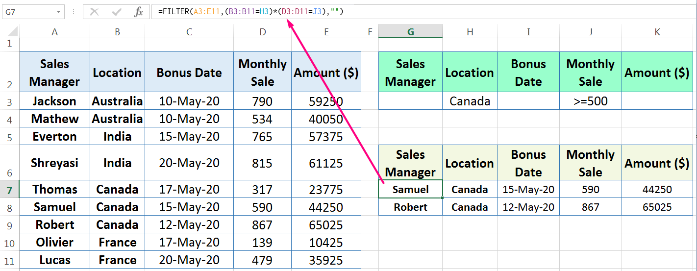
Similarly, we can use multiple AND criteria in the Excel Filter function. But keep in mind that in the include argument, each criterion should be surrounded by parenthesis and a multiplication operator (*) in between the criteria.
=FILTER(A3:E11, ((B3:B11=H3)*(D3:D11=J3),””)
(03) Examples of FILTER Function: Using Multiple OR Criteria
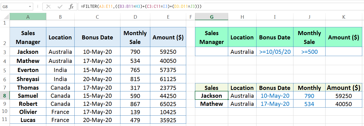
Simultaneously, we can use multiple OR criteria in the Excel Filter function. But in this case, in the include argument, each criterion should be surrounded by parenthesis and an addition operator (+) in between the criteria.
=FILTER(A3:E11, ((B3:B11=H3)+(C3:C11=I3)+(D3:D11=J3)))


Premium Courses on ed2go
Premium Courses on FutureLearn Limited
Premium Courses on Udemy
Premium Courses on Coursera

30+ BEST ADVANCE EXCEL COURSES | By Coursera, Udemy |
36+ BEST ADVANCED EXCEL COURSE ONLINE | By ed2go |
04 Best Ways : How to Use Multiple Columns VLOOKUP in Excel
04 Best Ways: How to Transpose Data in Excel
08 Best Examples of Excel Conditional Formatting
Tutorial 01: How to Use Excel SUMIFS Function with Single & Multiple Criteria
80+ Excel Shortcuts with ALT Key || Best Hotkey of Keyboard Shortcuts
Thanks for your interest joining to Advance Excel Forum community.
Something went wrong.

Join Our Community List
Subscribe to our mailing list and get interesting stuff and updates to your email inbox.
* VERIFY & CONFIRM YOUR EMAIL * We respect your privacy and take protecting it seriously*.


