5 years ago 3 years ago

BEST 05 WAYS: HOW TO CHANGE DATE FORMAT IN EXCEL?

by Sudipta Mondal 5 years ago3 years ago

5.8kviews

In Excel, it is mandatory to maintain a valid excel date format for making a project, data handling, and data analysis as well. Thus we must arrange the invalid Excel date format to a valid Excel date format such as ‘DD-MMM-YY’ (or any other valid date format) suggested by Excel.

But now the question arises in mind how to change the date format in Excel?

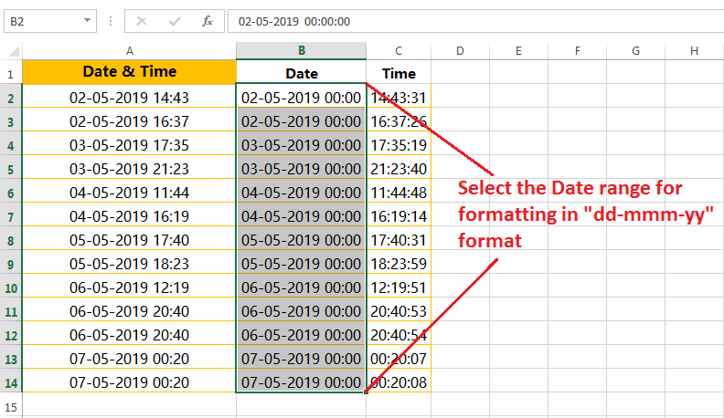
TABLE OF CONTENTS:

I. HOW TO CHANGE DATE FORMAT IN EXCEL?

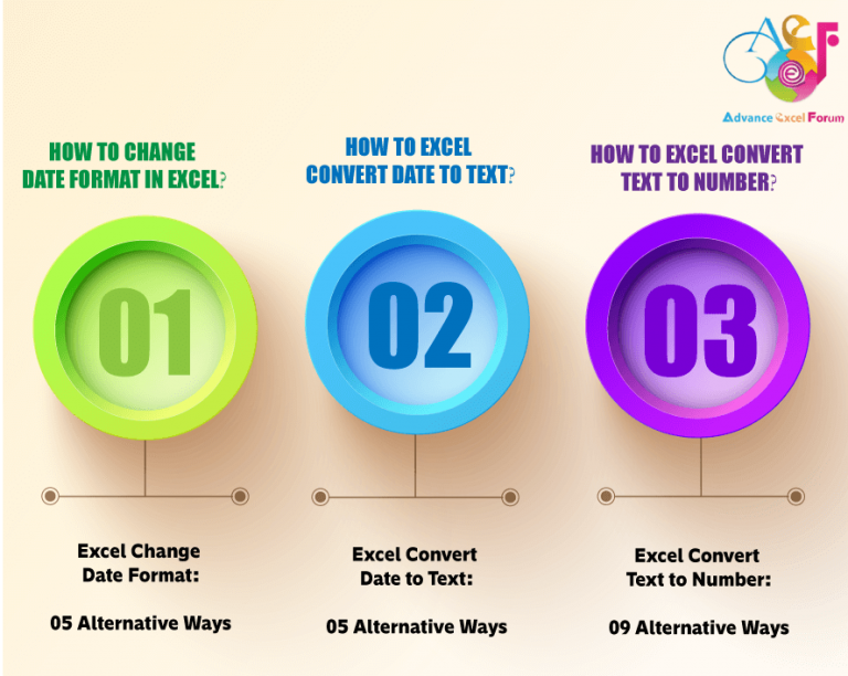
We can change the Excel date format in 5 ways:

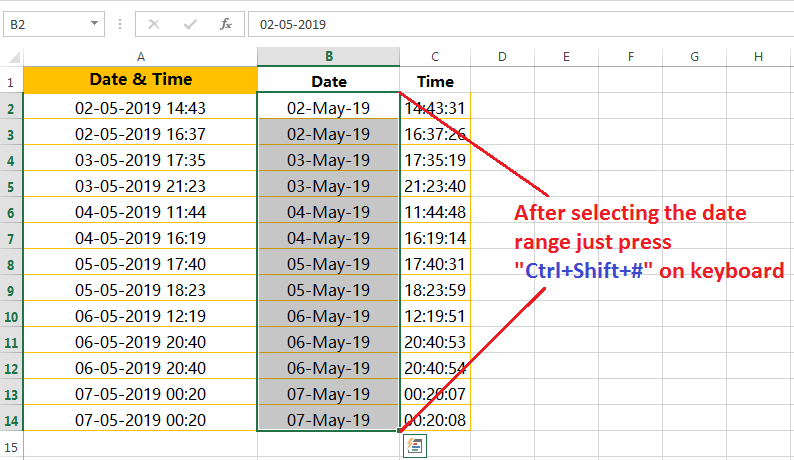
(01) CHANGE EXCEL DATE FORMAT: USING EXCEL SHORTCUT CTRL+SHIFT+#

Select the date range B2:B14 and then press Ctrl+Shit+#. All are arranged in a valid date format.

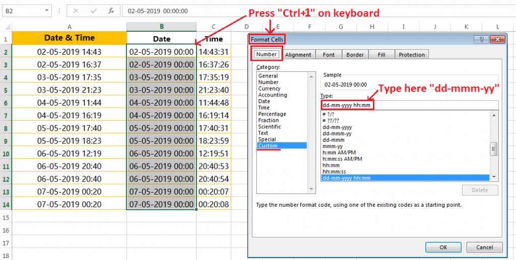
(02) CHANGE EXCEL DATE FORMAT: BY THE ‘FORMAT CELLS’ DIALOG BOX (USING EXCEL SHORTCUT CTRL+1)

Alternatively, select the data range B2:B14 ➪ then press ‘Ctrl+1‘ which will open the ‘Format Cells’ dialog box ➪ go to the ‘Custom‘ option under the Number tab ➪ On the right side, mentioned the required date format like dd-mmm-yy under the ‘Type‘ section.

(03) CHANGE EXCEL DATE FORMAT: BY THE ‘FORMAT CELLS’ DIALOG BOX (USING THE RIBBON)

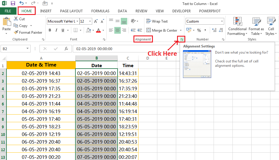
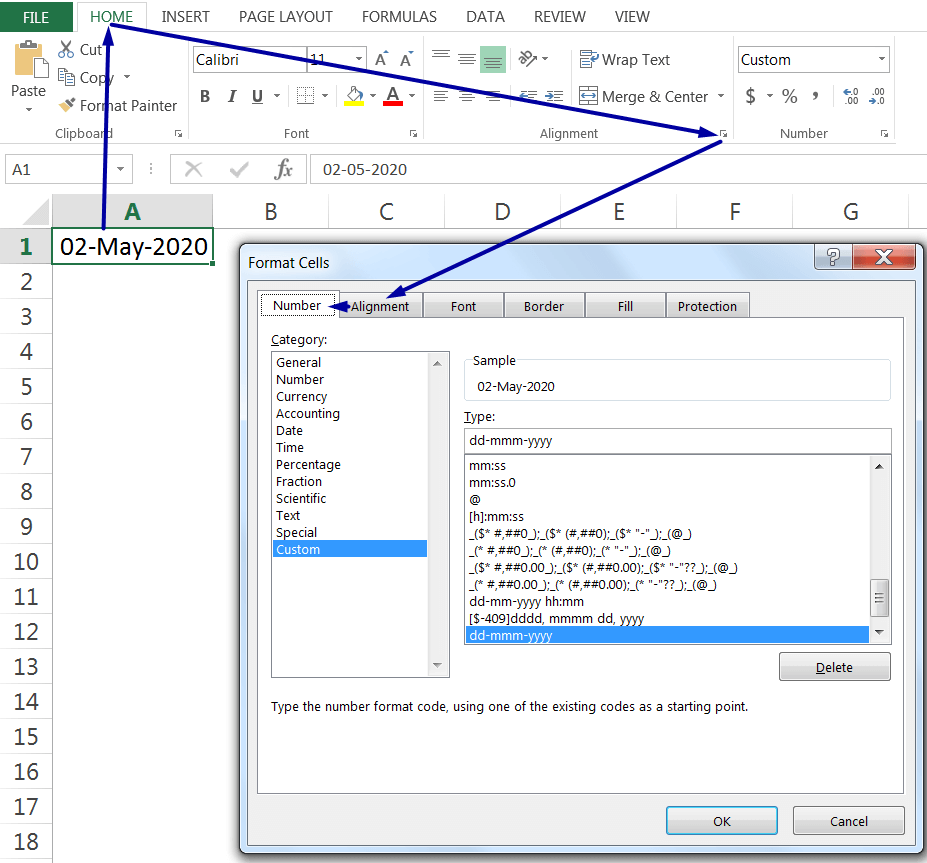
Alternatively, select the data range B2:B14 ➪ Go to the Home tab ➪ Click ‘dialog box launcher’ located on the right side corner of the ‘Alignment‘ group or ‘Number‘ group ➪ the Format Cells dialog box opens ➪ Select the ‘Custom‘ option under the Number tab ➪ On the right side, write the valid date format like dd-mmm-yy under the ‘Type‘ section.

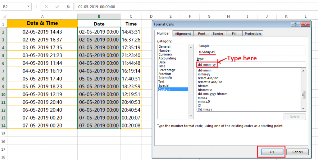
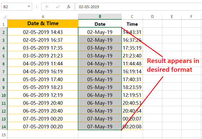
Finally, click OK or press Enter on the keyboard. We get the result in the desired date format as shown below:

(04) CHANGE EXCEL DATE FORMAT: USING THE ‘CONVERT TEXT TO COLUMNS’ WIZARD

The Convert Text to Columns Wizard is an advanced tool in Excel that helps to convert a range of varying date formats (such as text, number, invalid date format, valid date format etc.) to valid date formats.

➢ First, select the range of cells, i.e., A2:A14 ➪ then press Alt+D+E (sequentially Alt, D, E) or Alt+A+E (sequentially Alt, A, E) which will open the Convert Text to Columns Wizard.

• In Step 1 of 3, select ‘Delimited‘ (Excel by default select this option) ➪ then press ‘Enter‘ or click ‘Next‘.

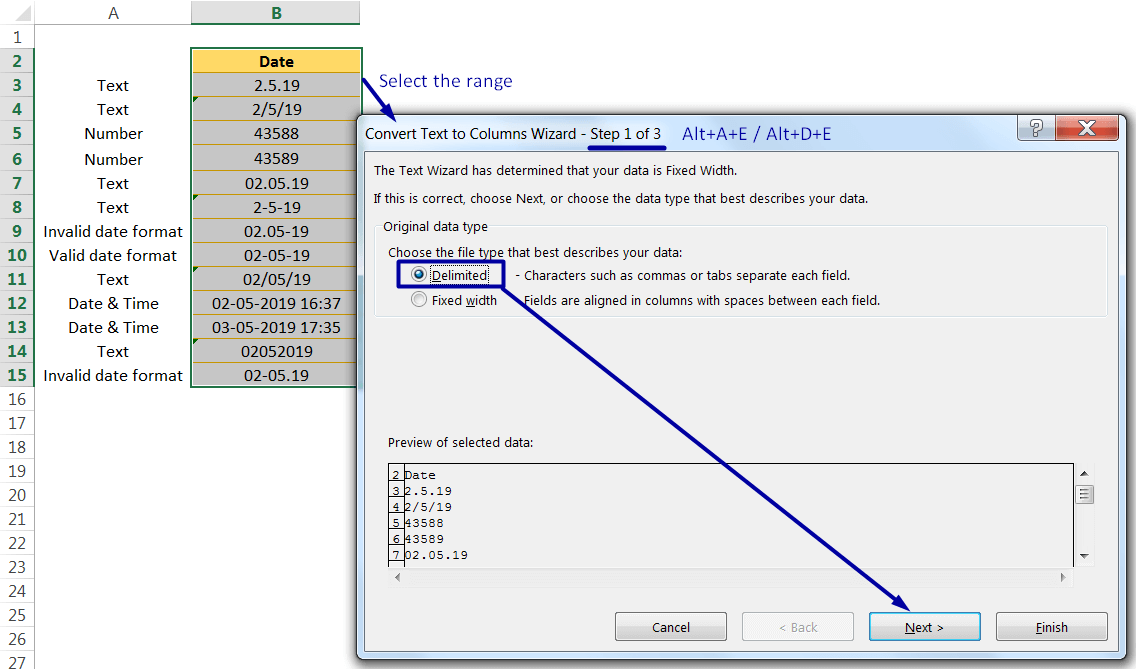
• In Step 2 of 3, uncheck all the checkboxes, if any (or, we can ignore the Tab checkbox) ➪ then press ‘Enter‘ or click ‘Next‘.

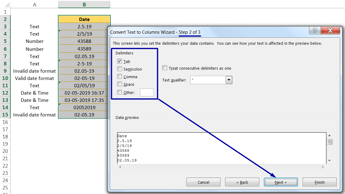
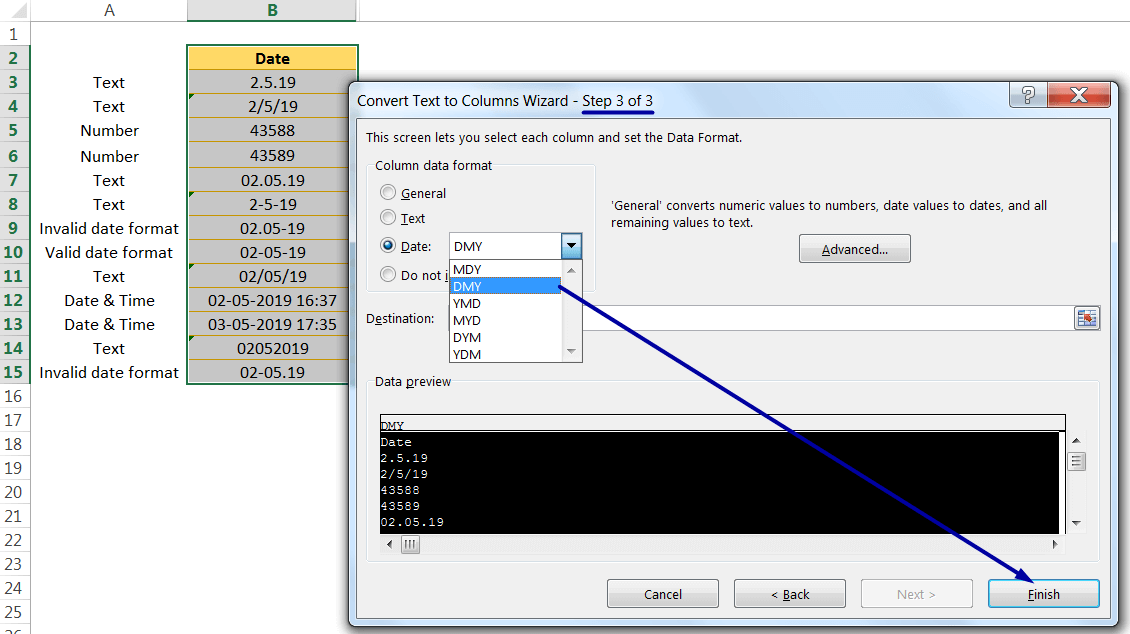
• In Step 3 of 3, select the ‘Date‘ option ➪ finally press ‘Enter‘ or click ‘Finish’.

➢ After applying the Text to columns, select the range again ➪ Then press Ctrl+Shift+# which allows us to convert numbers to valid Excel date format quickly.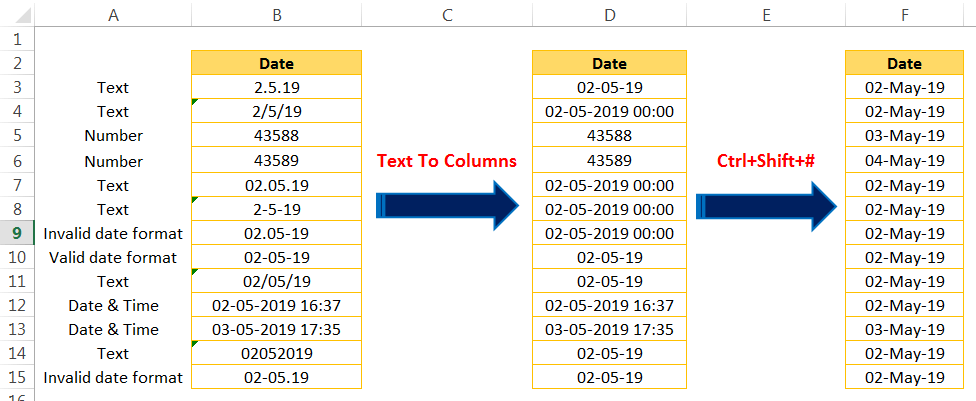

(05) CHANGE EXCEL DATE FORMAT: USING THE ‘CUSTOM FORMATTING’

Excel gives us a great deal of flexibility in creating custom date formats. When we create a custom date format, it can be used to format any cells in the workbook. We can create as many custom date formats as we need with the help of the codes used to create custom formats for dates and times.

HOW TO APPLY EXCEL CUSTOM DATE FORMAT?

We can apply the Excel custom date format with the ‘Custom’ category in the ‘Format Cells’ dialog box.

There are 06 ways to launch the Format Cells Dialog box, as explained below:

(01) Select the cell(s) ➪ Press Ctrl+1 on the keyboard which will open the ‘Format Cells’ dialog box ➪ Click the ‘Custom’ category on the ‘Number’ tab ➪Type the desired formatting code in the ‘Type:’ box or select the predefined formatting code from the below list.

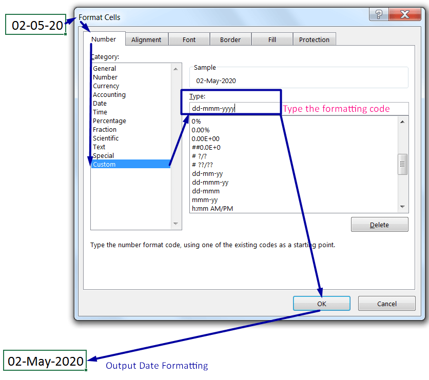
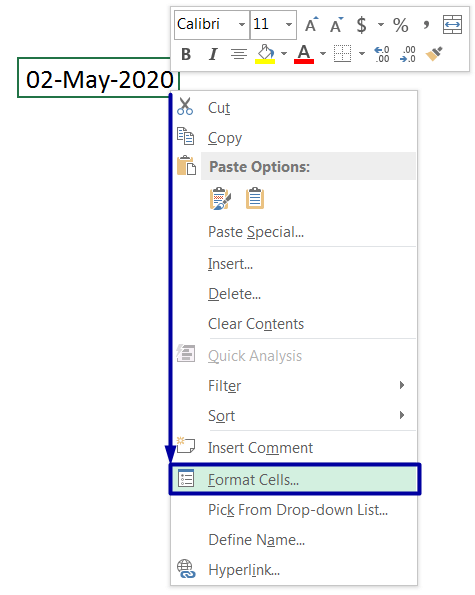
(02) Right-click the selected cell(s) and then select Format Cells which will open the ‘Format Cells’ dialog box ➪ Click the ‘Custom’ category on the ‘Number’ tab.

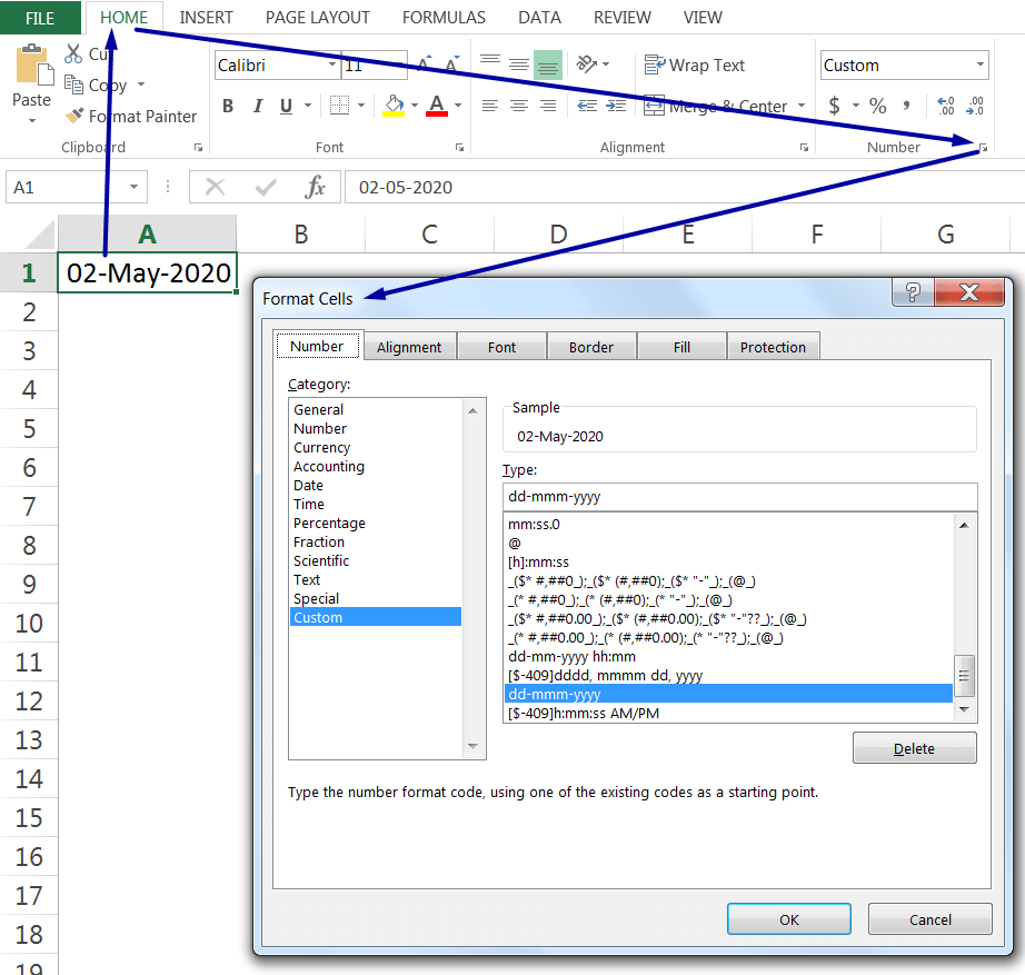
(03) Go to the Home tab ➪ Click the Number dialog box launcher, a small downward diagonal arrow, located at the bottom right corner of the Number group which will open the ‘Format Cells’ dialog box ➪ Click the ‘Custom’ category on the ‘Number’ tab.

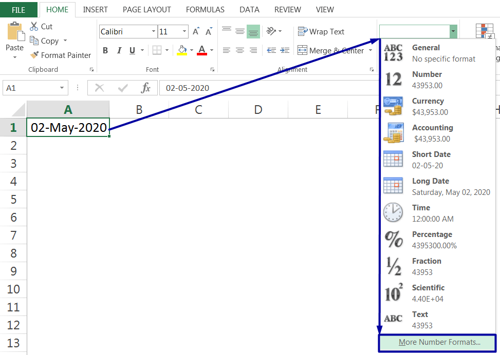
(04) Go to the Home tab ➪Click the Number Format drop-down in the Number group ➪ then click ‘More Number Formats’ located at the bottom of the list, which will open the ‘Format Cells’ dialog box ➪ Click the ‘Custom’ category on the ‘Number’ tab.

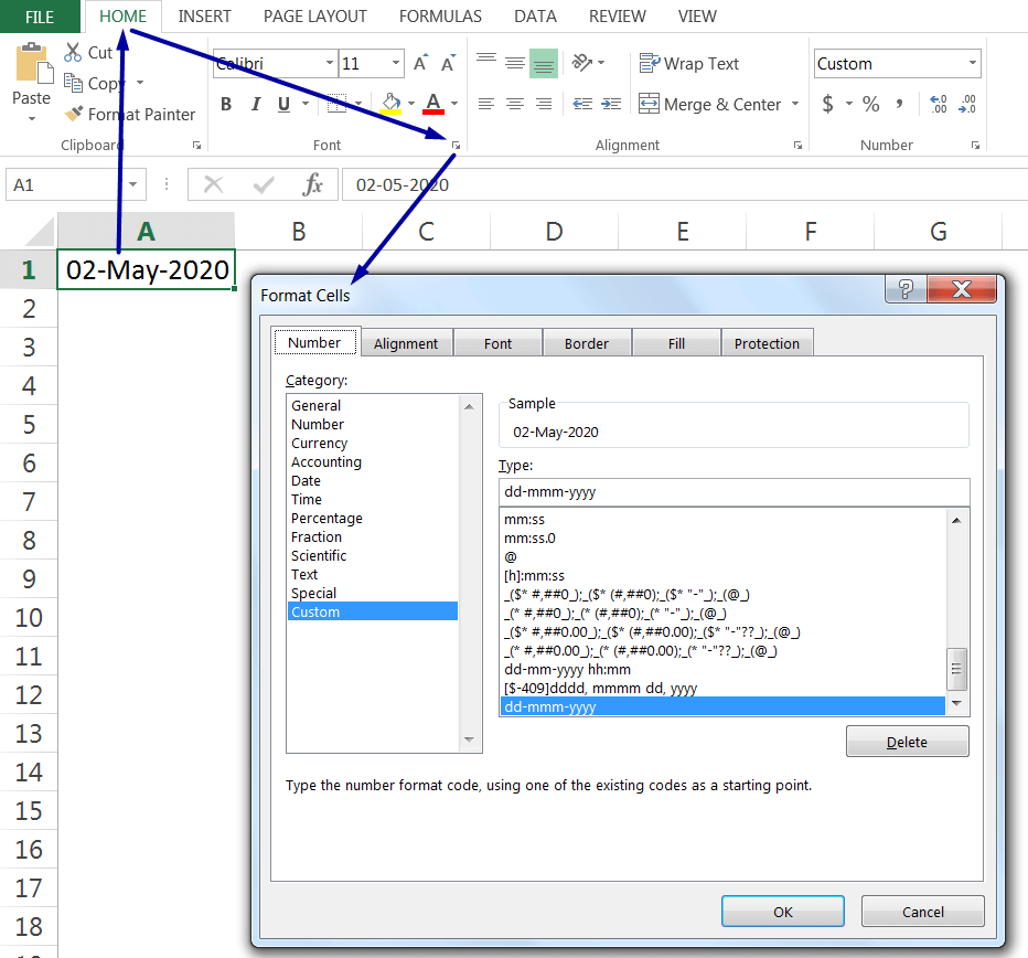
(05) Go to the Home tab ➪ Click the Font dialog box launcher located at the bottom right corner of the Font group ➪ ‘Font’ tab in the Format Cells dialog box opens then move to the ‘Number’ tab by clicking on it ➪ Click the ‘Custom’ category on the ‘Number’ tab.

(06) Go to the Home tab ➪ Click the command dialog box launcher located at the bottom right corner of the Alignment group ➪ ‘Alignment’ tab in the Format Cells dialog box opens then move to the ‘Number’ tab by clicking on it.

II. HOW TO EXCEL CONVERT DATE TO TEXT?

Sometimes it is required to convert a valid date format to a text format in Excel. We can follow any of the following methods:

(01) EXCEL CONVERT DATE TO TEXT: USING THE ‘CONVERT TEXT TO COLUMNS’ WIZARD

Steps to Start:

➢ At first, select the range of cells, i.e., A2:A14 ➪ then press Alt+D+E (sequentially Alt, D, E) or Alt+A+E (sequentially Alt, A, E) which will open the ‘Convert Text to Columns Wizard’.

• In Step 1 of 3, select ‘Delimited‘ (Excel by default select this option) ➪ then press ‘Enter‘ or click ‘Next‘.

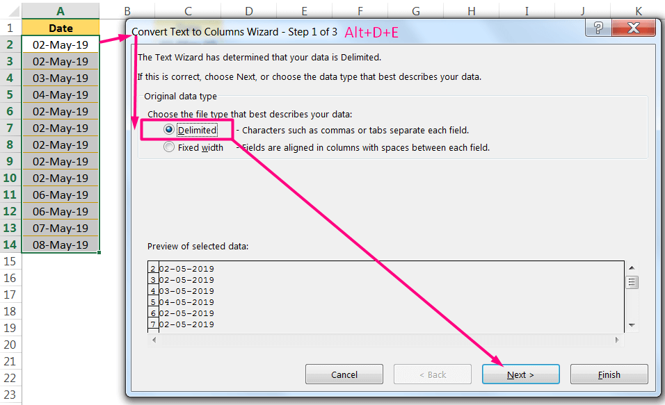
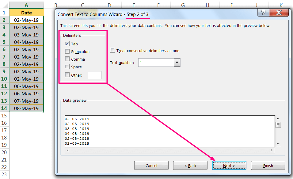
• In Step 2 of 3, uncheck all the checkboxes, if any (or, we can ignore the Tab checkbox) ➪ then press ‘Enter‘ or click ‘Next‘.

• In Step 3 of 3, select the ‘Text‘ option ➪ finally press ‘Enter‘ or click ‘Finish’.

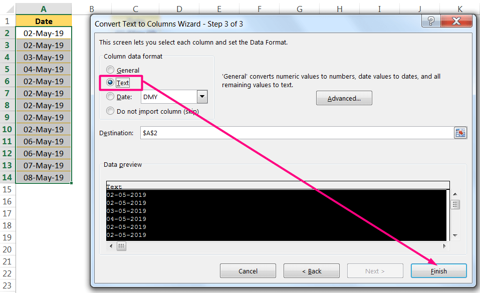
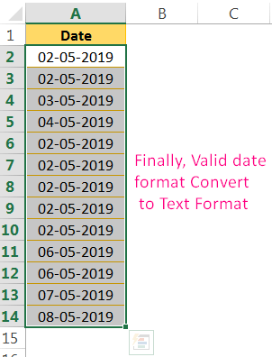
➢ As a result, the date format is converted to a text format, but without changing the date format.

(02) EXCEL CONVERT DATE TO TEXT: WITH THE ‘FORMAT CELLS’ DIALOG BOX (CTRL+1)

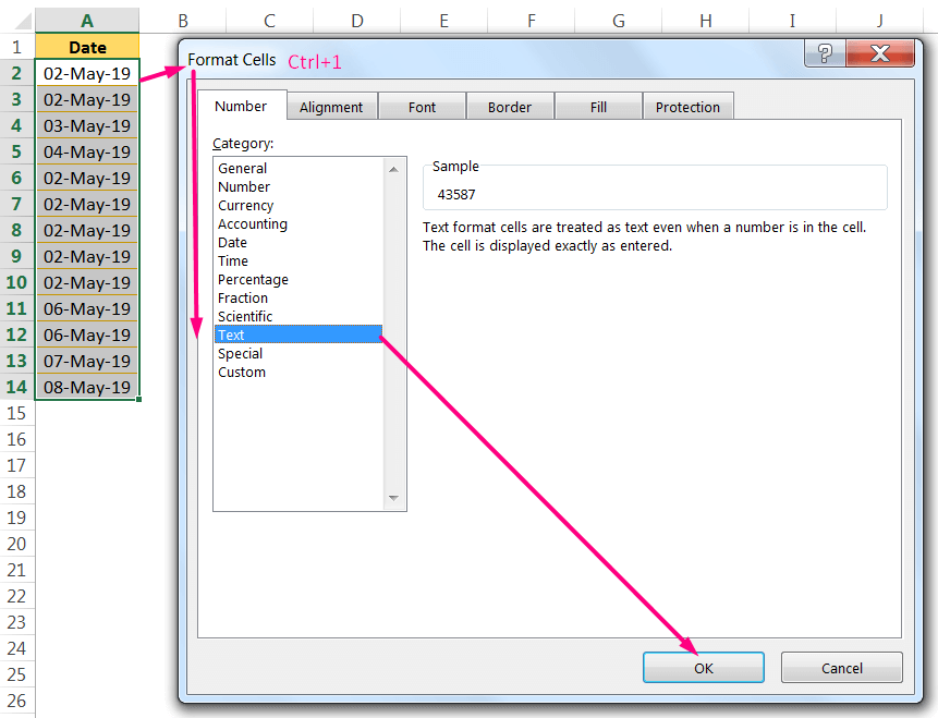
➢ At first, select the range of cells, i.e., A2:A14 ➪ then use Excel shortcut Ctrl+1 which will open the ‘Format Cells’ dialog box.

➢ In the second step, click on the ‘Number’ tab ➪ then select the ‘Text’ category ➪ finally press ‘Enter‘ or click ‘OK’.

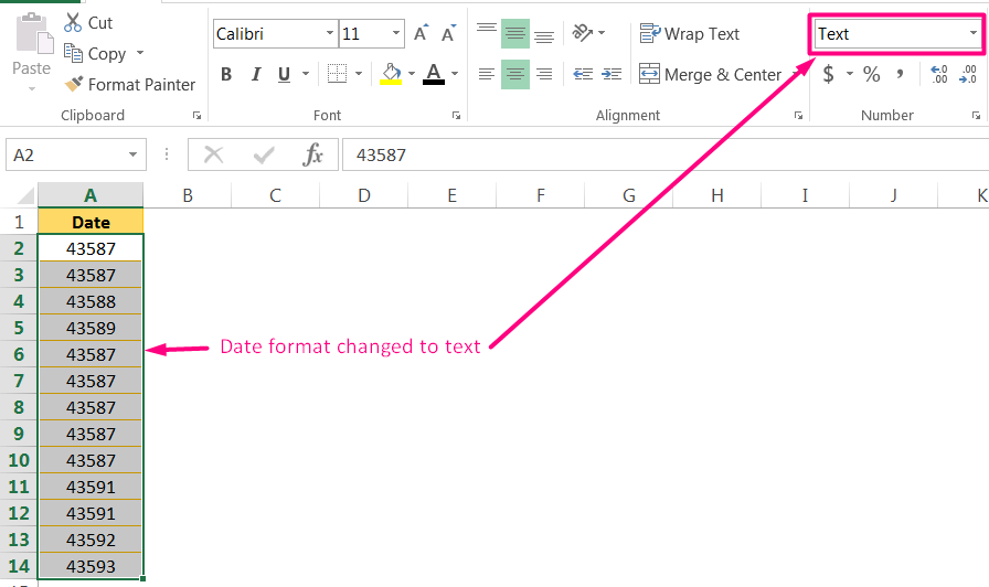
➢ As a result, the date format is converted to a text format where the date format changes to the general format.

(03) EXCEL CONVERT DATE TO TEXT: WITH THE ‘FORMAT BOX’ ON THE RIBBON (ALT+H+N)

➢ Method1: select the range of cells, i.e., A2:A14 ➪ then press Alt+H+N (sequentially press Alt, H, N) and type ‘te‘ which will select the ‘Text’ category in the format box of the ribbon ➪ then press ‘Enter‘ or ‘OK’.

Alternatively,

➢ Method2: select the range of cells, i.e., A2:A14 ➪ then press Alt+H+N (sequentially press Alt, H, N) which will select the format box of the ribbon ➪ then press Alt+⬇ (down arrow) which allows us to open a drop-down menu ➪ select the ‘Text’ category ➪ press ‘Enter‘ or ‘OK’.

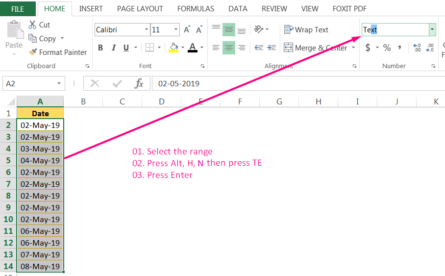
➢ As a result, the date format is converted to a text format where the date format changes to the general format.

(04) EXCEL CONVERT DATE TO TEXT: USING THE TEXT FORMULA

We can use the Excel TEXT function to convert a valid date format or numeric value to a text string.

The Syntax for the TEXT Function:

Arguments:

➢ value: It can be a numeric value, valid date format, a formula that returns a numeric value, or a cell reference contains a number. Value is the argument we want to convert to text.

➢ format_text: This argument defines how to format the input value argument as a text. Remember that the mentioned text format should be enclosed in double quotation marks.

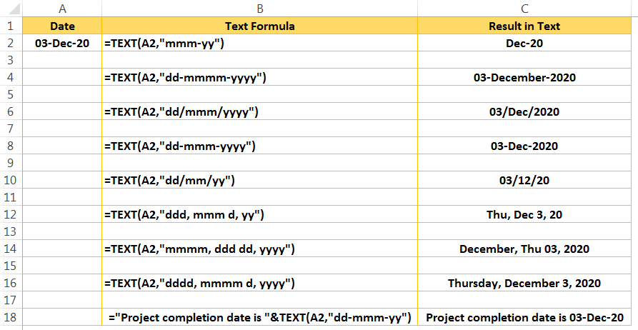
Using a set of date codes, we can format a date any way we like.

Note: We can separate the days, months, and year in date codes with various delimiters such as dash (-), slash (/), comma (,) colon (:), etc.

Example:

(05) EXCEL CONVERT CURRENT DATE TO TEXT: USING THE TEXT FORMULA

We can easily convert the current date to the text format using the TEXT function. In this case, we are using the TODAY function within the TEXT function. TODAY() function returns the current date. For example: =TEXT(TODAY(),”dd-mmm-yy”) and the formula returns the result as 03-Dec-20.

However, we can use the different format codes as per requirement.

III. HOW TO EXCEL CONVERT TEXT TO NUMBER?

Or, HOW TO CONVERT TEXT TO DATE IN EXCEL?

(01) EXCEL CONVERT TEXT TO NUMBER: USING THE TEXT FORMULA

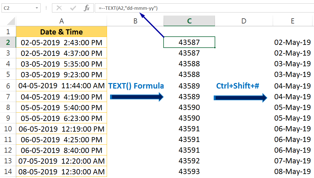
We can also use the Excel TEXT formula to convert text to number by adding double negation (–) prior to the TEXT formula and after the equality (=) sign.

For example, =—TEXT(A2,”dd-mmm-yy”)

After converting the number, press Ctrl+Shift+#which converts the number to date.

(02) EXCEL CONVERT TEXT TO NUMBER: USING THE INT FUNCTION

The INT function rounds a number down to the nearest integer, based on the value of the fractional part of the number.

The Syntax for the INT function:

➢ number: [Required] The number we want to round.

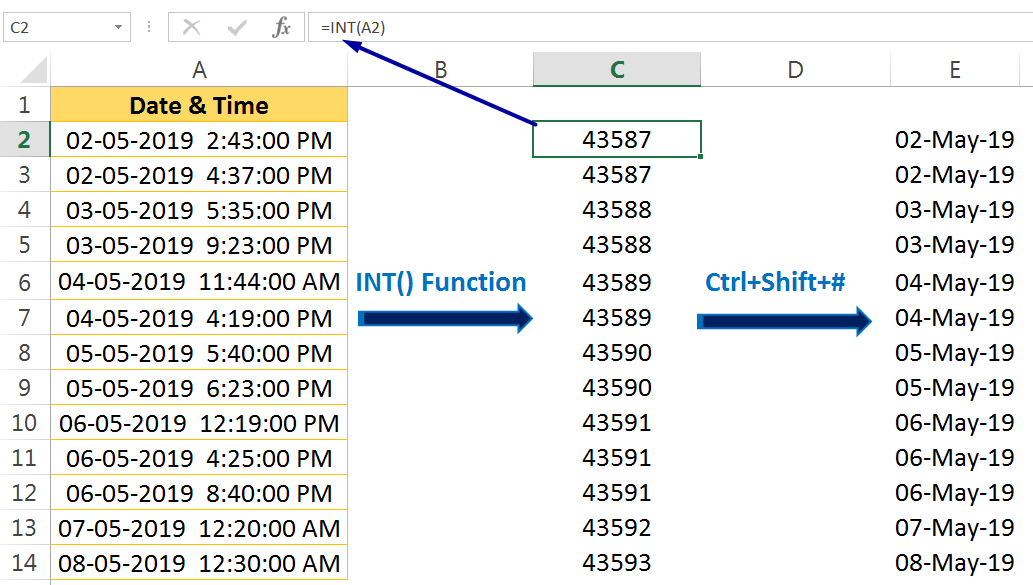
In the given example, the INT function is applied in cell C2.

=INT(A2)

The formula returns the result 43587.

Then copy the formula till the end of the range.

Finally, convert the formula into values with the help of Paste Special dialog box.

(03) EXCEL CONVERT TEXT TO NUMBER: USING THE TRUNC FUNCTION

Excel TRUNC function truncates a number to a specified number of significant digits. The TRUNC function simply removes the fractional part of a number.

The Syntax for the TRUNC function:

➢ number: [Required] The number we want to round or truncate.

➢ num_digits:[optional] This is a number that specifies the number of digits we want to truncate. If kept it blanks, it will take 0 as the default value.

num_digits Description:

> 0 (A positive value that is greater than zero): It specifies the number of digits truncates to the right of the decimal places.

0 (Equals to zero): It specifies the truncates all decimal places (this is the default)

< 0 (A negative value that is less than zero): It specifies the number of digits truncates to the left of the decimal places.

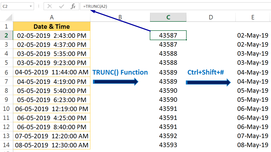
In the given example, the TRUNC function is applied in cell C2.

=TRUNC(A2)

The formula returns the result 43587.

Then copy the formula till the end of the range.

Finally, convert the formula into values with the help of Paste Special dialog box.

(04) EXCEL CONVERT TEXT TO NUMBER: USING THE EXCEL DATE FORMULA

The Excel Date formula is used to build a custom date by providing numbers or text string based on the year, month, and day provided.

A date consists of three components: the year, month, and day.

The Syntax for the Excel DATE Formula:

➢ year: This argument can be from one to four digits. Microsoft Excel for Windows uses the 1900 date system (a number between 1900 and 9999)

➢ month: A number representing the month of the year (1 to 12).

➢ day: A number representing the day of the month (1 to 31).

Note: If we enter a two-digit year, or even a three-digit year, Excel converts the number into a year value by adding 1900. Therefore, while we entering 10 as the year argument it gives 1910, not 2010. To avoid problems, always use a four-digit year when entering the DATE() function’s year argument.

Example 1:

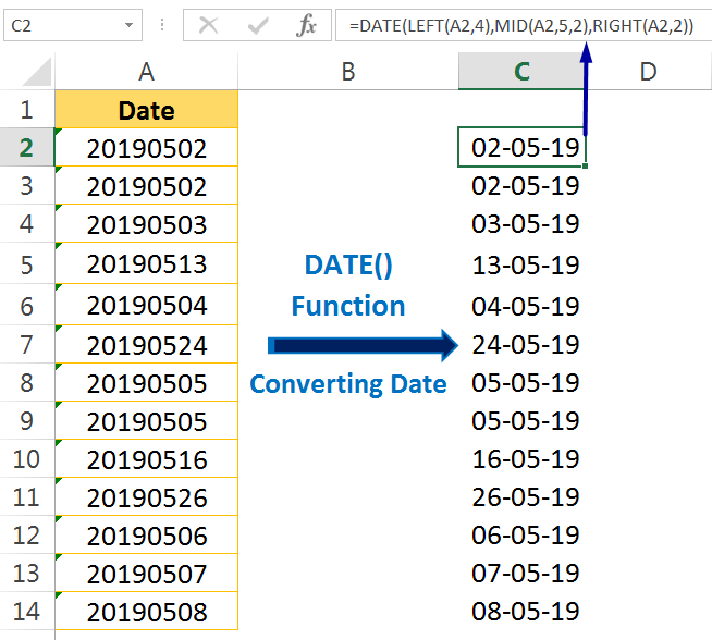
Sometimes dataset contains dates coded as text strings. For example, 20190502 – the text represents the date 02-May-2019 and the text is arranged in reversed order 2019-05-02 (a four-digit year followed by a two-digit month, followed by a two-digit day).

To convert this string to an actual date with the EXCEL DATE formula nested with text functions (LEFT, MID, and RIGHT).

• The LEFT() Function:

Returns the specified number of characters from the start of a text string.

The Syntax for the LEFT function:

➢ text: The original text or reference to a cell that contains the characters to be extracted.

➢ num_chars: The number of characters we want to extract from the left. The default value is 1.

For example, =LEFT(“20190502”, 4)

The formula returns 2019 (i.e., four characters from the left of a string).

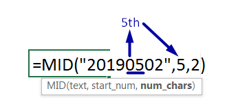
• The MID() Function

Returns the specified number of characters from the middle of a text string, based on a starting position and number of characters.

The Syntax for the RIGHT function:

➢ text: The original text or reference to a cell that contains the characters to be extracted.

➢ start_num: The character position in a string at which we want to start extracting the characters.

➢ num_chars: The number of characters we want to extract

For example, =MID(“20190502”, 5, 2)

The formula returns 05 (i.e., two characters from the middle of a string).

• The RIGHT() Function

Returns the specified number of characters from the end of a text string.

The Syntax for the RIGHT function:

➢ text: The original text or reference to a cell that contains the characters to be extracted.

➢ num_chars: The number of characters we want to extract from the right. The default value is 1.

For example, =RIGHT(“20190502”, 2)

The formula returns 02 (i.e., two characters from the right of a string).

Now, combine the formula in cell C2:

=DATE(LEFT(A2,4),MID(A2,5,2),RIGHT(A2,2))

➢ LEFT(A2,4) returns the Year 2019.

➢ MID(A2,5,2) returns the Month 05 (i.e. May).

➢ RIGHT(A2,2) returns the Day 02

After applying the formula press Ctrl+Enter or Enter key to apply the formula.

Then copy the formula till the end of the range.

Finally, convert the formula into values with the help of the Paste Special dialog box.

Example 2:

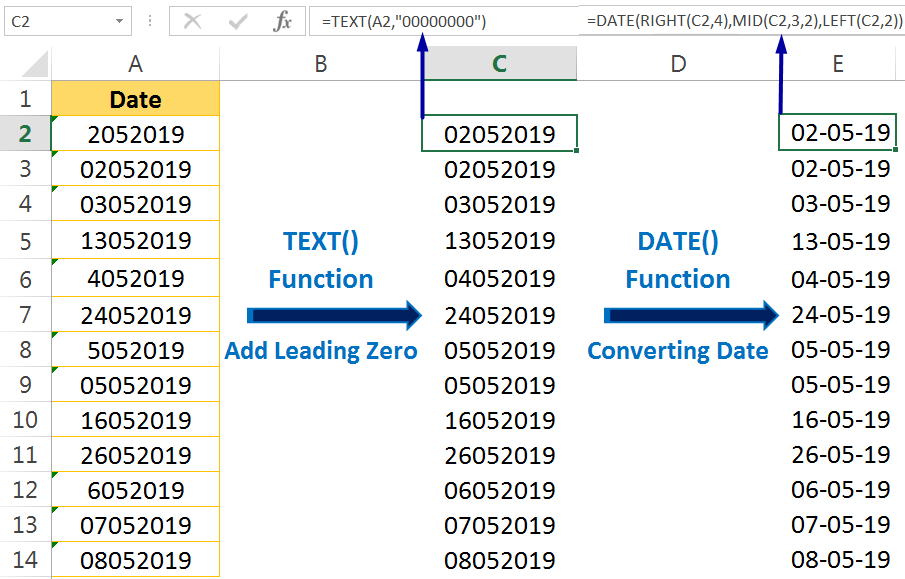
Sometimes, the date text format may be different (either use “D/MM/YYYY, “DD/MM/YYYY” or both can be used in a range).

Step 1: In this scenario, first we convert the range in “DD/MM/YYYY“ format with the help of the TEXT function. For example,

=TEXT(A2,”00000000“)

Step 2: In the second step, combine the TEXT functions (LEFT, MID, and RIGHT) in the DATE function to make a nested formula.

For example,

=DATE(RIGHT(C2,4),MID(C2,3,2),LEFT(C2,2))

➢ RIGHT(C2,4) returns the Year 2019.

➢ MID(C2,3,2) returns the Month 05 (i.e. May).

➢ LEFT(C2,2) returns the Day 02

After applying the formula press Ctrl+Enter or Enter key to apply the formula.

Step 3: Then copy the formula till the end of the range.

Step 4: Finally, convert the formula into values with the help of the Paste Special dialog box.

(05) EXCEL CONVERT TEXT TO NUMBER: USING THE DATEVALUE FUNCTION

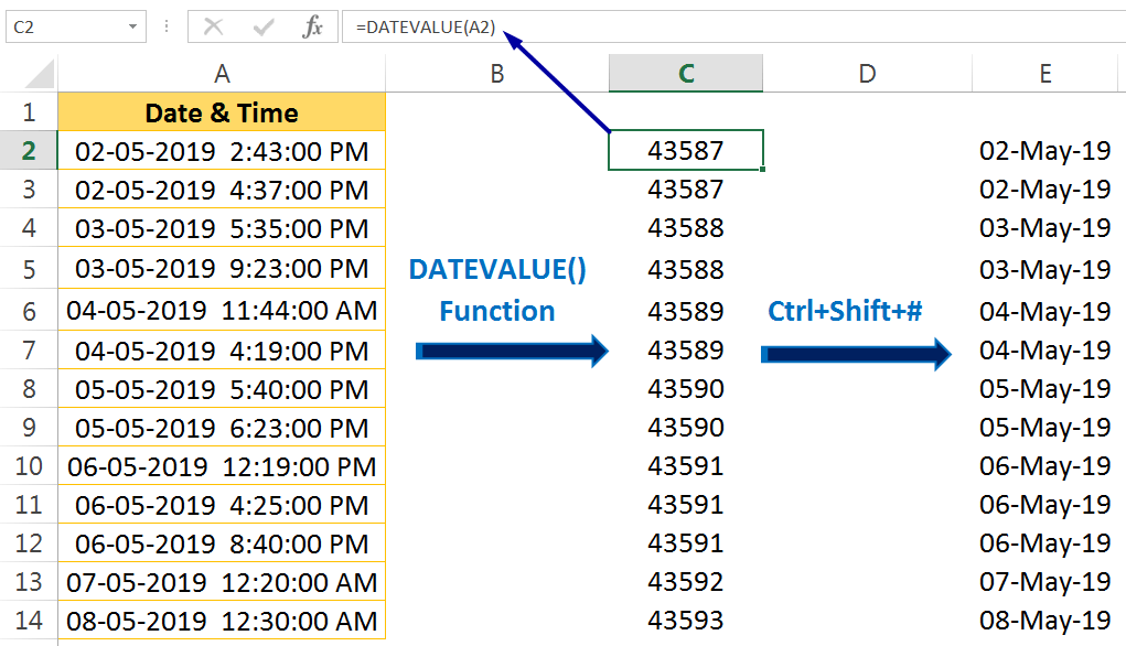
DATEVALUE() function converts a date in the form of text to a serial number. This formula ignores the time part convert to a serial number which means it only converts the day part of a date to a serial number excluding the time part.

The syntax for the DATEVALUE function:

➢ date_text: The string or cell reference containing the date.

The following formula returns 43587, the date serial number for 02.05.2019 2:43:00 PM. This formula simply ignores time to include in the result.

=DATEVALUE(“02.05.2019 2:43:00 PM”)

Using cell reference:

=DATEVALUE(A2)

After applying the formula in a cell, extends it to the entire range.

To view the result of this formula as a date, we need to apply a date number format to the cell. Generally, we select the cell or range of cells and press the keyboard shortcut Ctrl+Shift+#.

(06) EXCEL CONVERT TEXT TO NUMBER: USING THE SUBSTITUTE FUNCTION

In some situations, we may need the formula to replace a part of a text string with some other text. In this case, we use the Excel SUBSTITUTE function. The SUBSTITUTE function substitutes or replaces old text with new text in a text string.

The syntax for the SUBSTITUTE function:

➢ text: The original text or reference to a cell that contains the characters to be substituted.

➢ old_text: the text to be replaced

➢ new_text: the text we want to replace with old_text.

➢ instance_num: It specifies which occurrence of old_text we want to replace with new_text. When instance_num is specified, only that instance is changed. If we do not include instance_num, all occurrences are changed.

In the given example, we may need to convert the full stop (.) character to some other character likes hyphen (-) with the SUBSTITUTE function.

We wrap the SUBSTITUTE function either with the VALUE function or the DATEVALUE function.

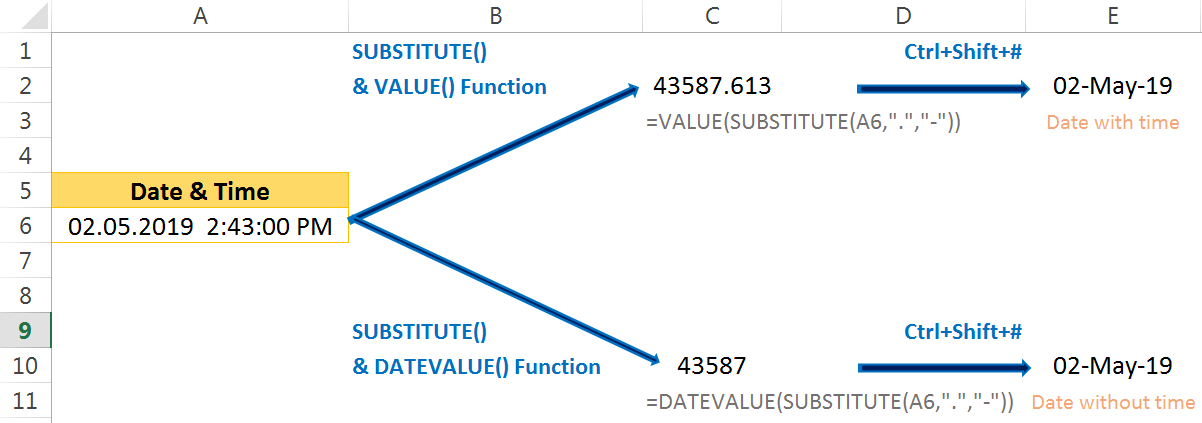
• DATEVALUE() function converts a date in the form of text to a serial number where it only converts the ‘day’ part in date to a serial number except the ‘time’ part.

The syntax for the DATEVALUE function:

➢ date_text: The original text or reference to a cell that contains the date text.

=DATEVALUE(“02.05.2019 2:43:00 PM”)

The formula returns the result:43587

When we wrap the SUBSTITUTE function and use the cell reference, it looks like:

=DATEVALUE(SUBSTITUTE(A6,”.”,”-“))

This formula signifies that the SUBSTITUTE function replaces full stop ”.” from cell content in cell A6 with a hyphen “-“. Then DATEVALUE function converts a date text string (the only daypart) into a date serial number and returns the result 43587.

To view the result of this formula as a date, we need to apply a date number format to the cell. Generally, we select the cell or range of cells and press the keyboard shortcut Ctrl+Shift+#.

• VALUE() function converts a date in the form of text to a numeric number. This formula includes the time into the numeric number as decimal places.

The syntax for the VALUE function:

➢ text: The original text or reference to a cell that contains the characters.

The following formula returns 43587.613, the date serial number for 02.05.2019 2:43:00 PM. This formula allows time to include in the result.

=VALUE(“02.05.2019 2:43:00 PM”)

When we wrap the SUBSTITUTE function and use the cell reference, it looks like:

=VALUE(SUBSTITUTE(A6,”.”,”-“))

This formula suggests that the SUBSTITUTE function replaces full stop ”.” from cell content in cell A6 with a hyphen “-“. Then the VALUE function converts a date text string (both day and time parts) into a numeric number and returns the result 43587.613.

Finally, convert this number to a date format (DD-MMM-YY) with the help of the keyboard shortcut Ctrl+Shift+#.

Note: In the case of a date where both day and time measured, we always prefer to apply the DATEVALUE() function instead of the VALUE() function to avoid the time part.

(07) EXCEL CONVERT TEXT TO NUMBER: USING THE CONCATENATE FUNCTION

CONCATENATE function is a text function that joins between 2 and 255 individual text strings into one text string.

➢ In the given example, we use DAY(), MONTH(), YEAR() functions and joined them with CONCATENATE() function. All the functions make a nested formula and return a text date format.

=CONCATENATE(DAY(A2),”/”,MONTH(A2),”/”,YEAR(A2))

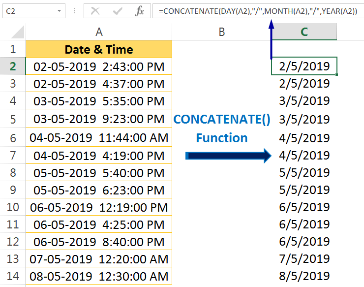
➢ Extend the formula till the end of the range (till cell C14).

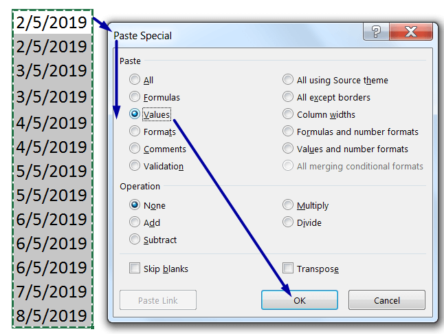
➢ Convert the formula into Values

Method 1: Select and copy the range (C2:C14) ➪ press Alt+E+S+V (sequentially press Alt, E, S, V) or press Alt+Ctrl+V+V (Alt+Ctrl+V, then V) which will select the ‘Values‘ option in the ‘Paste Special‘ dialog box ➪ Press Enter or click Ok.

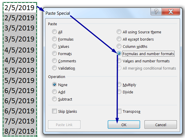
Method 2: Equivalently, Select and copy the range (C2:C14) ➪ press Alt+E+S+U (sequentially press Alt, E, S, U) or press Alt+Ctrl+V+U (Alt+Ctrl+V, then U) which will select the ‘Values and number formats‘ option in the ‘Paste Special’ dialog box ➪ Press Enter or click Ok.

➢ Convert Text to Date Format (Using Text to Columns)

This is a crucial step to convert text to date.

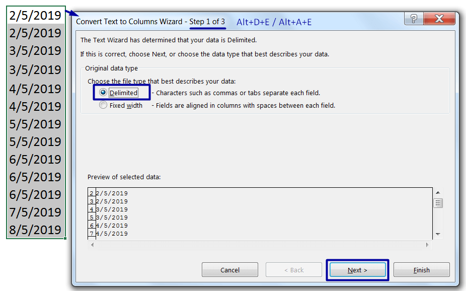
Select the range and press Alt+D+E (sequentially press Alt, D, E) or Alt+A+E (sequentially press Alt, A, E) which will open the ‘Convert Text to Columns Wizard‘.

• In Step 1 of 3, select ‘Delimited‘ (Excel by default select this option) ➪ then press ‘Enter‘ or click ‘Next‘.

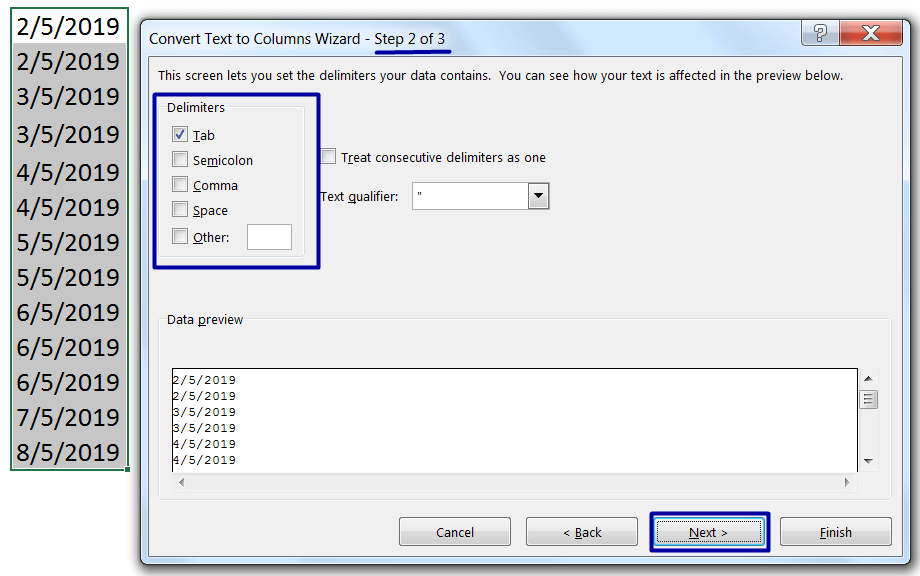
• In Step 2 of 3, uncheck all the checkboxes, if any (or, we can ignore the Tab checkbox) ➪ then press ‘Enter‘ or click ‘Next‘.

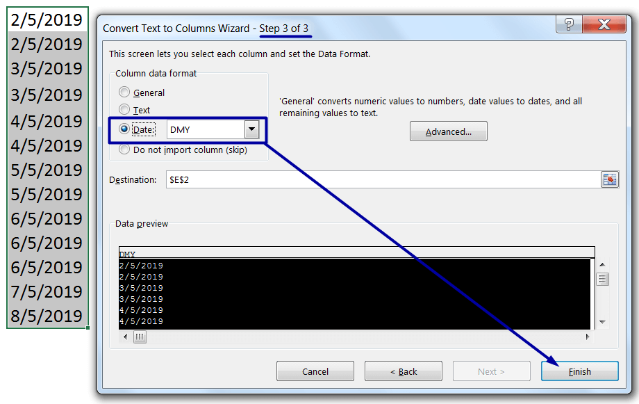
• In Step 3 of 3, Excel by default selects the ‘General‘ option ➪ Then press ‘Enter‘ or click ‘Next‘.

Equivalently, selects the ‘Date‘ option ➪ then press ‘Enter‘ or click ‘Next‘.

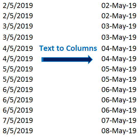
➢ As a result, the text date format is converted to a valid date format.

(08) EXCEL CONVERT TEXT TO NUMBER: USING THE DAY, MONTH, YEAR COMBINED FUNCTION

We can create a valid DATE format by joining DAY(), MONTH(), and YEAR() functions with the ampersand (&) symbol. Additionally, use a separator within double quotations (such as hyphen “-“, slash “/”) in between them.

=DAY(A2)&”/”&MONTH(A2)&”/”&YEAR(A2)

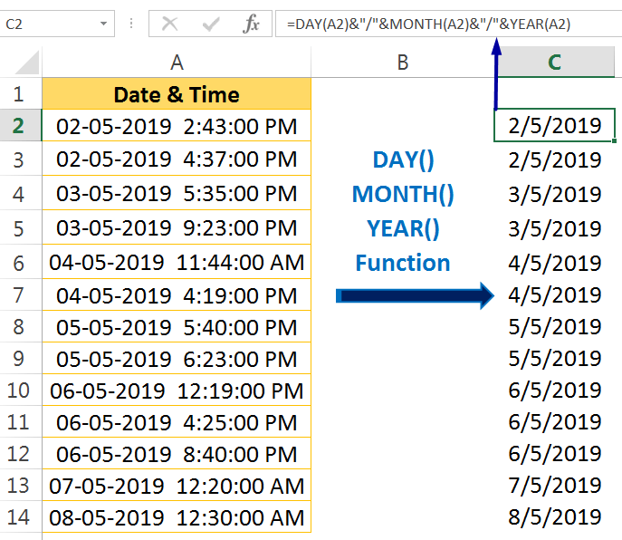
➢ Extend the formula till the end of the range (till cell C14).

➢ Convert the formula into Values.

➢ Convert Text to Date Format (Using Text to Columns)

(09) EXCEL CONVERT TEXT TO NUMBER: USING THE TEXT TO COLUMNS WIZARD

In the given example, first, we remove time from the date and simultaneously convert the text date to valid date format with the help of ‘Convert Text to Columns Wizard’.

➢ Select the range and press Alt+D+E (sequentially press Alt, D, E) or Alt+A+E (sequentially press Alt, A, E) which will open the ‘Convert Text to Columns Wizard‘.

• In Step 1 of 3, select ‘Delimited‘ (Excel by default select this option) ➪ then press ‘Enter‘ or click ‘Next‘.

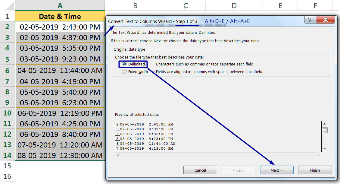
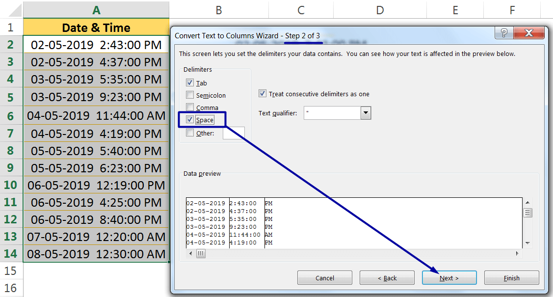
• In Step 2 of 3, select the ‘Space‘ checkbox as a delimiter ➪ Then press ‘Enter‘ or click ‘Next‘.

As a result, the date and time slot will be separated as display in the Data Preview section.

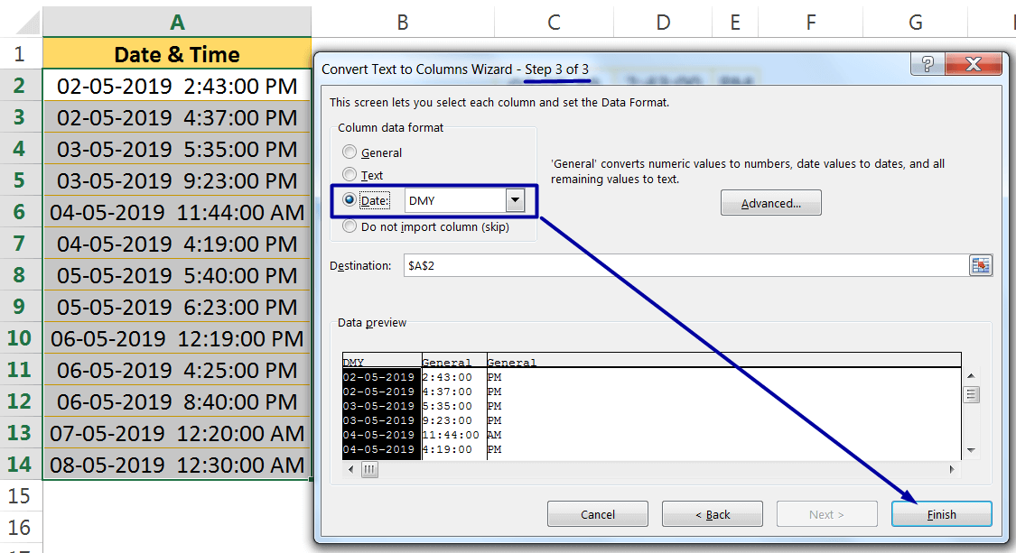
• In Step 3 of 3, select the ‘Date‘ radio-button, the Excel by default select ‘DMY’ format. If we want to select another format, then click on the drop-down and choose a desired format from the drop-down list ➪ Then press ‘Enter‘ or click ‘Finish‘.

As a result, date and time slots are split into different columns and additionally, text date format converted to valid date format.

If you would like to improve your academic and professional career as well, then the below courses help you a lot. Instead of Advanced Excel, a number of best courses suggested you through this platform that boosts your confidence and flies your career high.