Excel Definition & Learn Excel Spreadsheet

(01). EXCEL DEFINITION: WHAT IS EXCEL?

Excel is the well-known spreadsheet software used to store quantitative data and to perform accurate and rapid calculations and recalculations of data by using numerous built-in functions and formulas.

(02). WHAT IS AN EXCEL SPREADSHEET?

The Excel spreadsheet is a grid of cells organized into rows and columns in which we enter and store our data. Using Excel, we can create, edit, sort, analyze, summarize, and format data as well as graph it.

Additionally, the ribbon in Microsoft Excel is made up of a series of Command Tabs, each related to specific kinds of tasks that we perform in Excel. The Home tab is most often used by Excel users. However, each tab contains groups of commands, is called Command groups, related to specific tasks or functions.

Some commands have an arrow associated with them, is called Command Button Arrows / Command drop-down. This indicates that in addition to the default task, other options are available for the task.

Similarly, some of the Command groups have Dialog Box Launchers associated with them. Clicking on these displays additional commands not shown on the ribbon. Generally, the Clipboard, Font, Alignment, and Number groups have dialog box launchers or task panes, whereas Styles, Cells, and Editing do not.    

The new workbook contains one worksheet (Sheet1) by default where we enter information.

(03). EXCEL DEFINITION: WHAT IS AN ADVANCED EXCEL?

Excel has many inbuilt functions. Functions are predefined formulas that perform calculations by using specific values, called arguments, in a particular order, or structure. (Definition of argument: The value(s) that a function uses to perform operations or calculations is called an argument. The type of argument in a function is specific to the function. Common arguments that are used within functions include numbers, text, cell references, and names.)

When a number of functions combinedly make a nested function that creates a specific formula (i.e., an expression used to calculate a value) for performing a complex calculation based on multiple criteria is called Advanced Excel. Advanced Excel is a very necessary modern tool in the advanced world that can only be achieved through a committed focus and self-analysing skills. 

(04). INTRODUCTION TO EXCEL SPREADSHEET

I. EXCEL FILE MENU

When clicked on the File menu button, Excel opens the Backstage view, which contains a bunch of file-related options including Info, New, Open, Save, Save As, Print, Share, Export, Publish, Close, Account, and Options, which enables us to change Excel’s default settings. In this tutorial, we had mentioned below the most used options: 

➢ Info: Go to File ➪ Click Info in the Backstage view which will open the Info screen. On the left of the Info screen, we find the following commands:

• Protect Workbook – to encrypt the Excel workbook file with special access, such as a password, protect its contents, or verify contents of the file using a digital signature.

• Inspect Workbook – to check the document for metadata (data about the file) and see the file’s access options for people with disabilities and compatibility with earlier Excel versions.

• Manage Workbook – to recover or delete draft versions that are saved via AutoRecover

• Browser View Options – to manage parts of the Excel workbook that can be viewed or edited by users

• Properties – lists the size of the file as well as if there is any other info such as Title, Tags, or Categories dedicated to it. To add or edit this info, click the appropriate text box and start typing. To change additional file properties, we may click the Properties drop-down menu and click Show Document Panel from its drop-down menu.

• Related Dates – lists the date the file was in terms of Created, Last Modified, and Last Printed.

• Related People – lists names of the workbook’s author and other persons who last modified the file.

• The Show All Properties link – when clicked this expands the list of properties such as Comments, Template, Status, Subject, Categories, Hyperlink Base, and Company that can be edited.

➢ New: Go to File ➪ Click New ➪ Select Blank workbook which will open the new workbook.

Equivalently, using the Excel shortcut Ctrl+N.

➢ Open: Go to File ➪ Click Open ➪ Select existing workbook either of the three locations Recent Workbooks, OneDrive, Computer which will open the existing workbook.

Equivalently, using the Excel shortcut Ctrl+O.

➢ Save: Go to File ➪ Click Save which will save the modified existing workbook. For a new workbook, it helps to open the Save As dialog box.

Equivalently, using the Excel shortcut Ctrl+S.

➢ Save As: Go to File ➪ Click Save As ➪ Select a specific location (either Computer or OneDrive) or a specific folder by clicking the ‘Browse‘ folder at the rightside where we want to save the new file (workbook) ➪ A ‘Save As’ dialog box opens then type the valid ‘File name‘ and select the desired file type from ‘Save as type’ drop-down list. 

Equivalently, using the Excel shortcut Alt+F+A / Ctrl+F12 / F12.

➢ Print: Go to File ➪ Click Print which will open the Print Preview screen.

Equivalently, using the Excel shortcut Ctrl+P.

➢ Share: Go to File ➪ Click Share  ➪ Email ➪ Click ‘Send as Attachment‘ which will share a Excel file via outlook. 

Equivalently, using the Excel shortcut Alt+F+H+E+A.

➢ Close: Go to File ➪ Click Close which will close the current Excel File.

Equivalently, using the Excel shortcut Ctrl+W.

➢ Options: Go to File ➪ Click Options which allows us to change the Excel different options.

Equivalently, using the Excel shortcut Alt+F+T.

II. EXCEL TITLE BAR

This displays the name of the program and the name of the current workbook. It also holds the Quick Access toolbar (on the left) and some control buttons that you can use to modify the window (on the right).

➢ Quick Access Toolbar (QAT): The Quick Access Toolbar (QAT) is a shortcut tool for storing the commands we use most often and want quick access to. This toolbar consists of Autosave, Save, Undo, and Redo, it can also be Customized. AutoSave is automatically engaged after we first manually save a workbook to folder, desktop, drive, OneDrive or SharePoint website in the Cloud.

➢ Window Minimize Button: Click this button to minimize the workbook window. The window displays as an icon in the Windows taskbar

➢ Window Maximize / Restore Down Button: Click this button to increase the workbook window’s size to fill the entire screen. If the window is already maximized, clicking this button “unmaximizes” Excel’s window so that it no longer fills the entire screen.

➢ Window Close Button: Click this button to close the active workbook window.

III. EXCEL RIBBON / MENU BAR

At the top of the Excel window is a bar known as the Ribbon or Menu bar. The Excel Ribbon is the gateway to use Excel. It contains different tabs identified by unique names for easy identification and application. Each tab expands to show the various commands grouped within it. These commands can sometimes also be expanded. To select a command in a tab, click it. To select another tab, simply move the mouse away or use the excel shortcut. 

So the Excel ribbon or Menu bar is the tab-based user interface by which a user can navigate to the various features of Excel and can accomplish particular tasks.

Tabs are arranged in a series ranging from Home to View. The Excel Ribbon provides access to all of Excel’s capabilities and it contains the following seven tabs, proceeding from left to right:

(01) Home Tab: Use this tab when creating, formatting, and editing a spreadsheet. This tab is arranged into the Clipboard, Font, Alignment, Number, Styles, Cells, and Editing groups.

(02) Insert Tab: Use this tab when adding particular elements (including graphs, pivot tables, charts, hyperlinks, Symbols and headers and footers) to a spreadsheet. This tab is arranged into the Tables, Illustrations, Add-ins, Charts, Sparklines, Filter, Links, Text, and Symbol groups.

(03) Page Layout Tab: Select this tab to modify the overall look of a worksheet such as margins, orientation, colors, background and some print area settings.

 This tab is arranged into the Themes, Page Setup, Scale to Fit, Sheet Options, and Arrange groups.

(04) Formulas Tab: This tab contains all the formulas, formula error-checking tools, formula editing tools and Calculation Options.

This tab is arranged into the Function Library, Defined Names, Formula Auditing, and Calculation groups.

(05) Data Tab: All the data management and analysis commands are listed in this tab. We can also use this tab to sort and filter the data lists, Filter, Text to Columns, Data validation etc.

This tab is arranged into the Get External Data, Connections, Sort & Filter, Data Tools, and Outline groups.

(06) Review Tab: Use this tab for spell checking, protecting worksheet and workbook, and marking up a spreadsheet for review by others.

This tab is arranged into the Proofing, Language, Comments, and Change groups.

(07) View Tab: Use this tab when changing the display of the Worksheet area and the data it contains. It contains commands to hide/reveal the gridlines, zoom in /zoom out, freezing panes and more. This tab is arranged into the Workbook Views, Show, Zoom, Window, and Macros groups.

The above explained tabs are present by default in every ribbon. Some ribbons also contain additional tabs, resulting from activating macros and installing add-ins.

➢ Add-Ins Tab: The add-ins tab is visible in two scenarios,

(01) If we install any add-ins.

(02) If we open a workbook saved in the older version. Since the traditional menus are not present in Excel 2013, all these appear in the add-ins tab.

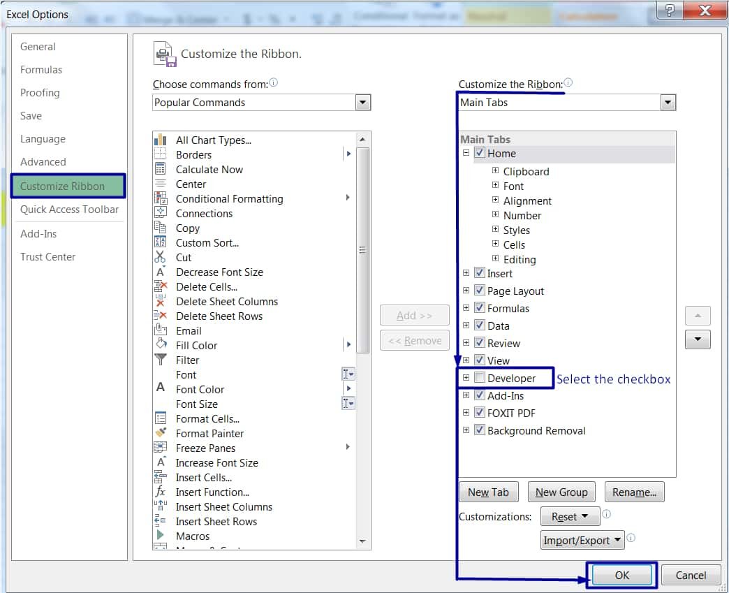
➢ Excel Developer Tab: This tab contains commands and tools that are normally used for advanced programming. The Developer Tab is hidden by default. If we want to make it visible, perform the following steps on Excel.

Go to the ‘File‘ tab ➪ Select Options  ➪ Choose Customize Ribbon from the left sidebar ➪ On the right side, we will find Customize the Ribbon section. Under this heading, there will be a Developer Checkbox and select the checkbox. This action added the Developer Tab on the Ribbon.

➢ Help: To display the Excel Help task pane, we just click the Help button that displays as a question mark in the top-right corner of the Title bar or press F1. The subsequent Help window will offer suggestions relevant to our task.

IV. EXCEL FORMULA BAR

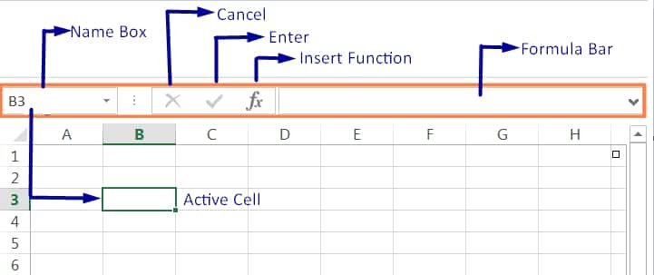
The formula bar in Excel is located at the top of the worksheet area, below the ribbon. The job of the formula bar is to display the formula or values (text or data) used in the active cell. In the active cell, Excel displays only the result of the formulas, not the formula itself. Sometimes, ranges and objects have names. When that is the case, the name appears instead of the address. By clicking the drop-down arrow next to the section that holds the addresses and names, we can see a list of all objects within the current workbook that have names. If the list is empty except for the address of the active cell, named objects are not currently used in that workbook.

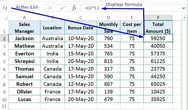
The Formula Bar has three parts, namely:

➢ Name box – the leftmost section that displays the address of the active cell. For example, if we click cell B3, B3 appears in the name box. If we click on another cell, the address for that cell then appears in the name box. 

➢ Formula Bar buttons – There are 03 buttons

• Cancel – When we enter or edit data, click Cancel to cancel the data entry or edit, and revert back to the previous data in the cell, if any. Cancel changes from grey to red when we position the pointer over it.

• Enter – When we enter or edit data, click Enter to accept data typed in the active cell and keep the current cell active. Enter changes from grey to blue when you position the pointer over it.

• Insert Function – Click to display the Insert Function dialog box to search for and select a function to insert into the active cell. The Insert Function icon changes from grey to green when we position the pointer over it.

➢ Formula Bar – the third section is the formula bar in Excel that takes up the rest of the bar and expands to display long cell entries that won’t fit in the normal area. The contents of the cell are completely editable. When the Cell contents area is blank, it means that it is empty.

V. EXCEL WORKSHEET AREA

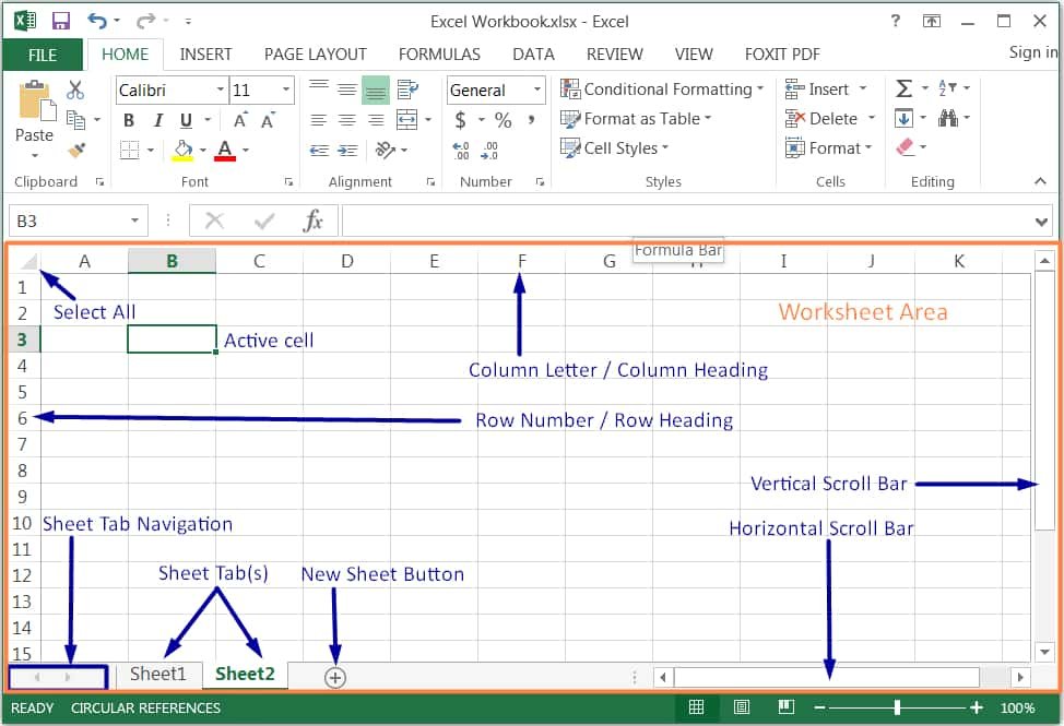
This area contains all the cells of the current worksheet.

A worksheet is a grid composed of rows, columns, and cells. Each worksheet column starts at the top of the worksheet and goes to the bottom of the worksheet and is identified by a letter. Each row starts at the left edge of the worksheet and continues to the right and is identified by a number. Each cell on the grid is identified by the intersection of a column and a row. Thus, the first cell in an open worksheet is A1, where “A” denotes column address and “1” denotes row number. 

We enter information by typing it into the selected cell or active cell, which is outlined by a bold rectangle. This is also called the current cell or highlighted cell.

Excel identifies a current cell by

(a) the green border surrounding the cell appears in the cell,

(b) the cell address appears in the Name box of the Formula bar,

(c) the current cell’s column letter and row number are shaded in the column and row headings.

The row number indicates what row we are on in the workbook. An Excel worksheet has a potential of 1,048,576 rows and 16,384 columns (XFD). Columns are identified by letters and rows by numeric values/numbers. This means that a single worksheet contains more than 17 billion cells. Each cell can hold 32,767 characters.

➢ Select All – The triangle at the intersection of the row and column headings in the top-left corner of the worksheet. Click it to select everything contained in the active worksheet.

➢ Column Headings / Column Letters – The letters above the columns, such as A, B. C…till XFD. For example, A is the letter above the first column, whereas C is above the third column. We can click a column letter to select an entire column of cells or drag a column border to change its width.

➢ Row Headings – The numbers to the left of the rows, such as 1, 2, 3, and so on. For example, 5 is the row heading for the fifth row. Similarly, we can select a row number and change its width.

➢ Scroll Bar – The vertical scroll bar and horizontal scroll bar allow us to move through the worksheet page. We use a horizontal scroll bar on the bottom to move left and right through the sheet and a vertical scroll bar on the right edge to move up and down through the sheet.

➢ Sheet Tab(s) – By default, Excel has a single sheet tab (Sheet1). Each of the different tabs represents a different sheet in the workbook. A workbook can have any number of sheets, and each sheet has its name displayed in a sheet tab.

➢ New Sheet Button – Click to insert a new worksheet to the right of the current worksheet.

➢ Sheet Tab Navigation – If the workbook contains several worksheets, Excel may not show all the sheet tabs at the same time. Use the buttons to display the first, previous, next, or last worksheet.

VI. EXCEL STATUS BAR

The Status bar in Excel is located at the bottom of the Excel worksheet area and displays information about the status of the active workbook. Normally, the Status bar will display the word Ready to indicate that the workbook is ready to be used. When cells are being edited, the Status bar will display Edit.

This bar informed us which program running currently, and any special keys we engage, and it also enables us to select a new worksheet view and to zoom in and out on the worksheet.

In addition to displaying information about the current status of the active workbook, the Status bar also displays information about Circular References. 

➢ View Controls – Icons on the right side of the status bar that control how we are viewing the worksheet. Click a view control to display the worksheet in Normal, Page Layout, or Page Break Preview.

• Normal view is the default view and it displays the worksheet without showing margins, headers, footers, and page breaks.

• Page Layout view shows the margins, header and footer area, and a ruler. Page Layout View shows how the page will look when it is printed. Use this function to ensure the printed workbook will be neat and easy to read.

• Page Break Preview indicates where the worksheet will be divided into pages.

• Zoom control allows us to increase or decrease the size (zoom percentage) of the worksheet on the screen.