How to Find And Replace in Excel? After entering data into the cells of a workbook or worksheet, we can find almost any values, text string, whether it is located in a cell, formula, cell reference, or range name with the help of the Find command in the Find and Replace dialog box. Once it is found, we have the option of replacing the text on a case-by-case basis or all at once using the Replace command in the Find and Replace dialog box.
The Excel Find and Replace dialog box includes a feature that allows us to search our worksheet to locate cells that contain specific formatting (for example, a currency symbol). This feature does not locate cells that contain formatting resulting from conditional formatting.
TABLE OF CONTENTS:
Toggle(A) HOW TO FIND A VALUE/TEXT USING FIND AND REPLACE IN EXCEL?
(01) HOW TO FIND A TEXT/NUMERIC VALUE FROM EXCEL WORKSHEET
We can find the text string within a specific range, or within the entire worksheet with the help of the ‘Find and Replace’ dialog box either in 2 ways:
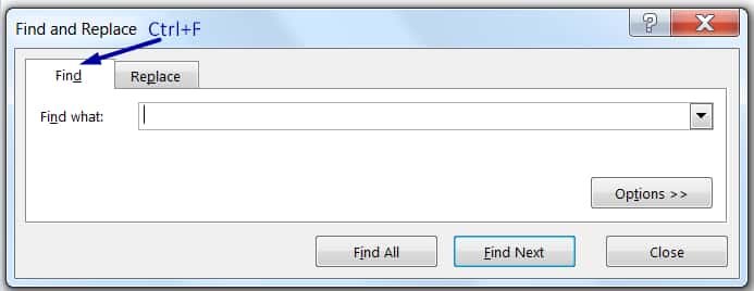
• Open ‘Find’ Dialog box Using the Excel Shortcut: Click any cell or select the entire range or select the specific cells from where to find the specific value or text ➪ then press Ctrl+F.
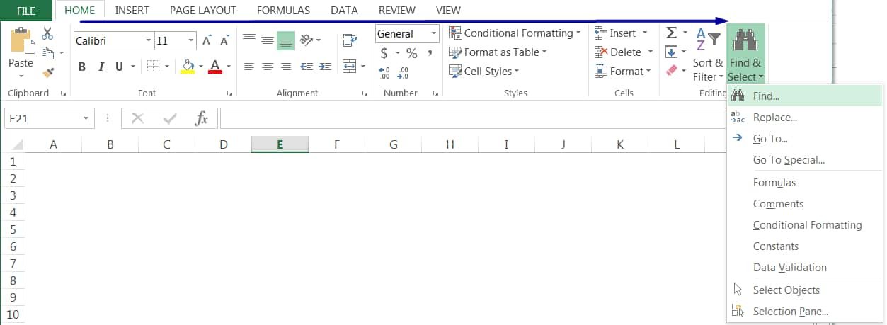
• Open ‘Find’ Dialog box Using the Ribbon: Click any cell or select the entire range or select the specific cells in the worksheet ➪ Go to the Home tab ➪ Click Find & Select drop-down in the Editing group ➪ Click Find.
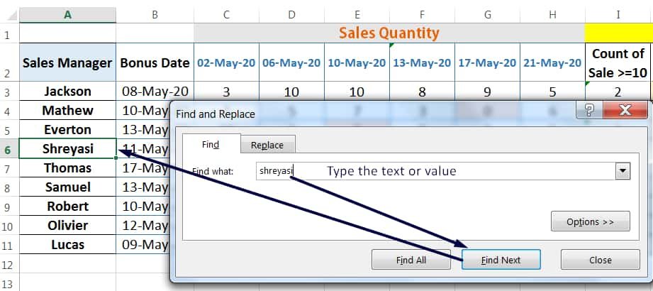
In the Find and Replace dialog box, enter the text string to find under the ‘Find what’ text box ➪ Either click Find All or Find Next ➪ Click Close or press Esc key.
(02) HOW TO FIND A TEXT/NUMERIC VALUE FROM EXCEL WORKBOOK
To search the entire workbook, we must select the Workbook from the drop-down list in the ‘Within’option.

(03) EXPLORE FIND AND REPLACE ADVANCED OPTIONS
■ Set the ‘Search’ option: Excel can search by columns or rows, however, by default it is selected ‘By Rows’ in the Search option. If it is selected by rows, Excel will begin searching in the current row and move across the entire row before dropping down to the next row. If it is selected by columns, Excel will begin searching in the entire current column and move to the next column to the right.
In either case, when the end of the worksheet is reached, Excel will continue searching from the beginning at cell A1 until it returns to the currently selected cell.
■ Set the ‘Look in’ Option: This is important and could not find any result if set incorrectly. The options as follows:
(i) Formulas: If we choose this option, Excel will search cells that begin with an equal sign (formula) as well as any constant values. However, the results of the formula will not be searched.
(ii) Values: In this case, Excel searches the calculated value and constant value, not the actual formula.
(iii) Comments: This checks cell comment only.
■ ‘Match case’: If we want to find an exact match, with the same use of upper- and lower- case letter then select the checkbox ‘Match Case’. Text strings that do not match exactly will be ignored.
For example, if we search with the name ‘thomas’ it will find ‘thomas’, ‘thomas singing a song.’ from the list, but it ignores the rest because this option allows a case-sensitive search.

■ ‘Match entire cell contents’: If we checked this option Excel finds entire cell contents and will only find a match if there are no other extraneous chracters or numbers in the cell. In this option, upper- and lower- case letters do not matter at all.
For example, if we search with name ‘thomas’ it will find ‘thomas’, ‘Thomas’, ‘THOMAS’ from the list but it ignores the cell with other extraneous characters.

(04) FIND CONTENT USING WILDCARDS CHARACTERS
The wildcard characters asterisk (*) and question mark (?) can be used to expand the search.
The Asterisk (*) symbol is used to replace any number of characters. For example, to find all occurrences of the word total, use *Total*. This will find Total, Sub total, Subtotal, Totals, Grand Total.

Likewise, the question mark (?) is used to find a single character. For example, ?total would find Sub total, Subtotal, Grand Total.

(05) FIND CONTENT IN CELLS WITH SPECIFIC FORMAT
To find content in cells with the specific format by Find and Replace dialog box.
• Press Ctrl+F which will open the Find and Replace dialog box.
• Click Options >> in the lower right corner.

• Then click the Format… drop-down in the upper right corner and select Choose Format From Cell…

• As a result, a color picker with an addition symbol will activate. Then select a cell with specific formatting which will command Excel to isolate all the cells with the same formatting.
• Click Find All.

(B) HOW TO REPLACE A VALUE/TEXT USING FIND AND REPLACE IN EXCEL?
Replace option helps to find and replace the values and text strings in formulas or constant values. It cannot find and replace the results of a calculation.
Note: Be extremely careful with the ‘Replace All’ button as it can have a significant effect on the worksheet, potentially replacing text that we may not want to be changed. Thus, it is the best practice to select the range prior to invoking the ‘Find and Replace’ command, then Replace All will only affect the selected range.
(01) HOW TO REPLACE A TEXT/NUMERIC VALUE FROM EXCEL WORKSHEET
• Open ‘Replace‘ Dialog box Using the Excel Shortcut: Click any cell or select the entire range or select the specific cells in the worksheet ➪ then press Ctrl+H.
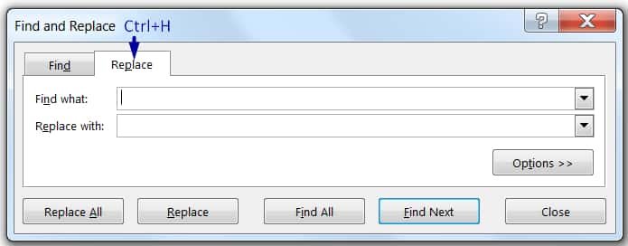
Equivalently, Select the range of cells ➪ Then press Ctrl+F. The ‘Find and Replace’ dialog box will be displayed ➪ Then click on the ‘Replace’ button.
• Open ‘Replace’ Dialog box Using the Ribbon: Click any cell or select the entire range or select the specific cells in the worksheet ➪ Go to the Home tab ➪ Click Find & Select drop-down in the Editing group ➪ Click Find.
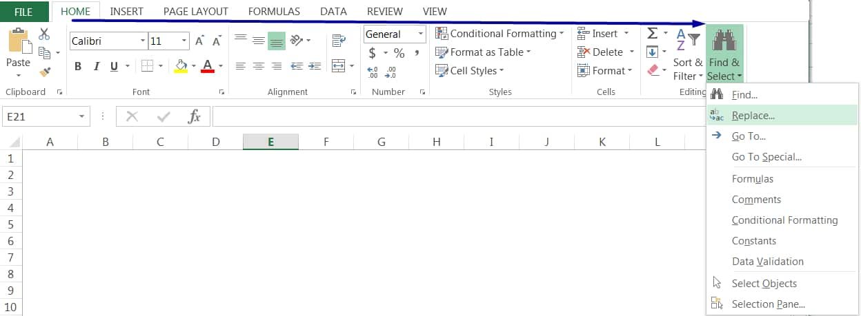
For example, to replace the existing text or value with the desired text or value from a worksheet we should follow the following steps:
• Either select a specific range of the dataset or the entire dataset.
• Then press Ctrl+H which will open the Replace tab in the Find and Replace dialog box.
• Type the existing text in front of the ‘Find what:’ box. For example, type the text #n/a.
• Type the replaceable text in front of the ‘Replace with:’ box. For example, type zero (0).
• Click Replace All. As a result, all the text #N/a is replaced with the value 0 from the worksheet.
• After replacing, press the Esc key or click Close.

(02) HOW TO REPLACE A TEXT/NUMERIC VALUE FROM EXCEL WORKBOOK
To replace the existing text or value with the desired text or value from all the worksheets in a workbook, we must select the Workbook from the drop-down in the ‘Within’option.

• Place cursor in a worksheet, then press Ctrl+H which will open the Replace tab in the Find and Replace dialog box.
• Type the existing text in front of the ‘Find what:’ box. For example, type the text #n/a.
• Type the replaceable text in front of the ‘Replace with:’ box. For example, type zero (0).
• Click Options >> at the below of the right corner and as a result, more advanced settings will open. Then select the Workbook from the drop-down in the ‘Within’option.
• Click Replace All. As a result, all the text #N/a is replaced with the value 0 from all the worksheets in a workbook.
• After replacing, press the Esc key or click Close.
➢ Key Points To Note:
• In the ‘Find what’ text box, type the text that we want to replace. For example, here we want to replace all the #N/A Errors.
• In the ‘Replace with’ text box, type the new text that will take the position in place of the existing text. For example, here we place 0 (zero) value which means all the #N/A Errors will be replaced by 0.
• Click Replace All button to replace all the text string from the entire worksheet at a time.
• Click Replace to replace the text string in the single selected cell.
• Click Find All to find the text string from the entire worksheet.
• Click Find Next to skip this instance of the text and move to the next time it occurs.
When Excel can find no more occurrences of the text, it will alert us with a message. Choose the Close button or press the Esc key to end our search.
(03) HOW TO FIND AND REPLACE A LINE BREAK IN EXCEL
We can easily insert a line break in Excel’s cell by pressing Alt+Enter. But it is very difficult to remove a line break manually one by one from a huge dataset.
It is easiest to use Find and Replace to replace a line break with a space or any separator (likes slash”/”, dash “-“, etc.).
(i) At first, press Ctrl+H which will open the Find and Replace dialog box.
(ii) Then Press Ctrl+J in the ‘Find what:‘ field. [Ctrl+J denotes the ASCII control code for character 10 (line break, or line feed].
(iii) Then enter a space by pressing the Spacebar key once in the ‘ Replace with:‘ field.
(iv) Finally, click Replace All. As a result, all the line breaks will be replaced with spaces in a worksheet.

(04) EASY TO CHANGE CELL FORMATTING WITH FIND AND REPLACE
In Excel, we can easily change the same cell formatting with the Find and Replace dialog box.
(i) Press Ctrl+H which will open the Find and Replace dialog box ➪ Click the Options.
(ii) Click the Format drop-down located in front of the ‘Find What:’ box ➪ Click Choose Format from Cell ➪ Select a cell with the desired cell formatting. Selected cell formatting is shown in the Preview section.

(iii) Similarly, click the Format drop-down located in front of the ‘Replace with:‘ box ➪ Click either Choose Format from Cell or Format (where to apply own desired format). Selected cell formatting is shown in the Preview section.
(iv) Finally, click Replace All. As a result, similar cell formatting will be replaced with the new cell formatting in a worksheet.
If we want to apply the change in the entire workbook, then we select the Workbook option in the ‘Within’ drop-down box.


Premium Courses on ed2go
Premium Courses on Coursera
Premium Courses on Udemy

30+ BEST ADVANCE EXCEL COURSES | By Coursera, Udemy |
36+ BEST ADVANCED EXCEL COURSE ONLINE | By ed2go |
80+ Excel Shortcuts with ALT Key || Best Hotkey of Keyboard Shortcuts
03 Useful Methods : Add Numbers With AutoSum Excel
04 Simple to Advanced Methods: How to Filter in Excel?
05 Best Ways: Create Password Protect Excel & Unprotect it
08 Best Examples: How to Use Excel Conditional Formatting?
04 BEST WAYS: HOW TO TRANSPOSE DATA IN EXCEL
Tutorial 01: How to Use Excel SUMIFS Function with Single & Multiple Criteria
Thanks for your interest joining to Advance Excel Forum community.
Something went wrong.

Join Our Community List
Subscribe to our mailing list and get interesting stuff and updates to your email inbox.
* VERIFY & CONFIRM YOUR EMAIL * We respect your privacy and take protecting it seriously*.


