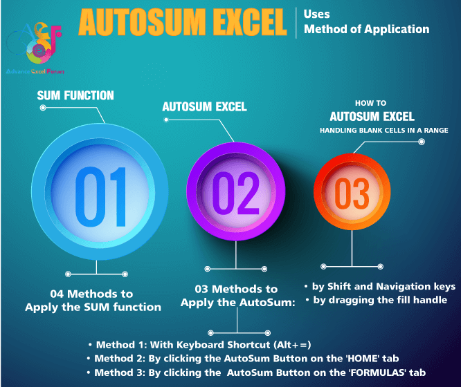
One of the most popular functions available in Excel is the AutoSum function. Excel AutoSum automatically totals the contents of cells.
Excel AutoSum is a formula that calculates (by default) the total from the adjacent cell up to the first non-numeric cell using the SUM() function in its formula. The AutoSum feature provides a quick way to sum a contiguous range of numbers (that means there are no empty cells in a range). The range may be a single cell or thousands of cells.
The AutoSum icon is the Greek capital letter Sigma ∑. Math and Science use the Sigma ∑ as a summation operator.
TABLE OF CONTENTS:
Toggle01. HOW TO USE SUM FUNCTION IN EXCEL?
The SUM function is a mathematical function in Excel that totals values in one or more cells in a range and displays the result in the cell containing the function. It is applicable for both contiguous and non-contiguous cells or ranges.
In the case of contiguous cells or ranges, select them by the dragging of the mouse or by the Shift and navigation arrows.
For non-contiguous cells or ranges, hold the CTRL-key and select them by dragging the mouse.
The syntax for the SUM function: number1, number2,… The values we want to add
Note: Brackets [ ] indicate optional arguments; however, do not actually type the brackets when we enter the argument.
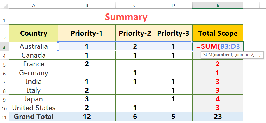
The SUM function contains one required argument (number1) that represents a range of cells to add. For example, =SUM(B3:D3). Excel will sum all cells within that range.
We can enter up to 255 arguments into the SUM() function. For example, the following formula returns the sum of the values in three separate ranges: =SUM(B3:D3,B7:D7,B10:D10).
We can apply the SUM Function in a cell with 03 different methods:
• Method 1: Apply SUM Function With ‘Formula AutoComplete Tool’
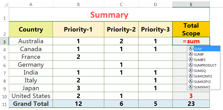
(01) Select the cell where to apply SUM function ➪ place equality sign (=) and type sum, Excel by default select the SUM function from the drop-down list; otherwise select the SUM function with down navigation arrow (⬇).
Note that the upper or lower case does not matter for syntax, Excel by default considers it in upper case.
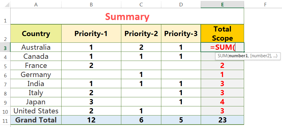
(02) Then press the Tab key which allows us to open the SUM function with an open parenthesis.
(03) Select the range.
(04) Then press Ctrl+Enter or Enter to accept the formula.
• Method 2: Apply SUM Function With ‘Insert Function’ dialog box
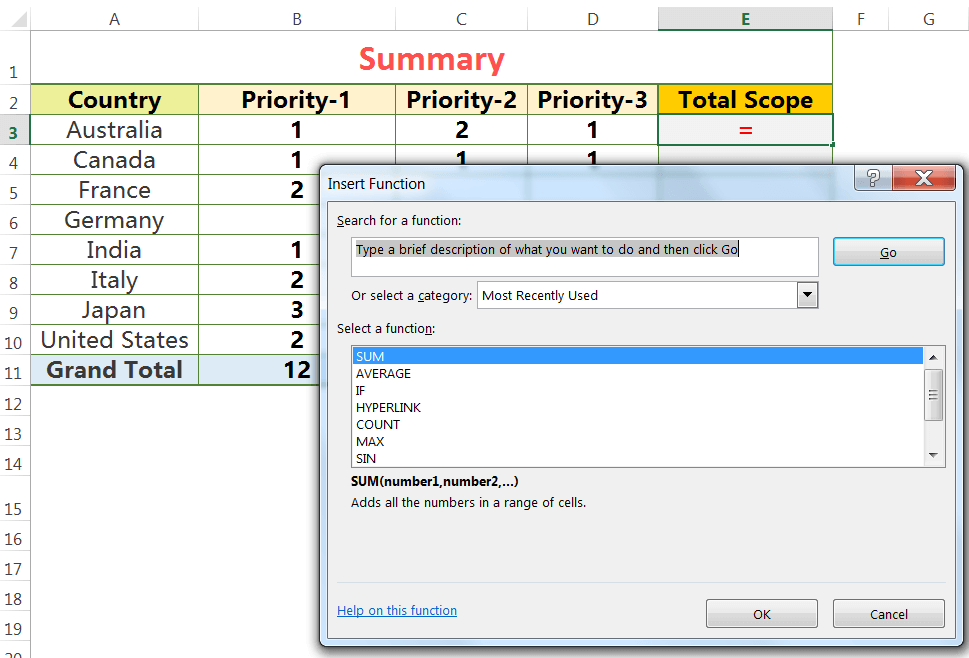
(01) Select the cell where to apply the SUM function.
(02) Press Shift+F3 which will open the ‘Insert Function’ dialog box. Excel automatically places an equal sign (=) in the cell.
➢ Type and Search SUM function in ‘Search for a function:’ box ➪ then click OK or,
➢ Click to choose a category from ‘Or select a category:’ drop-down list, for example, select ‘Math & Trig’ category and find the SUM function using the horizontal scroll bar ➪ then click OK.
Note: Excel’s built-in functions are grouped into ten categories.
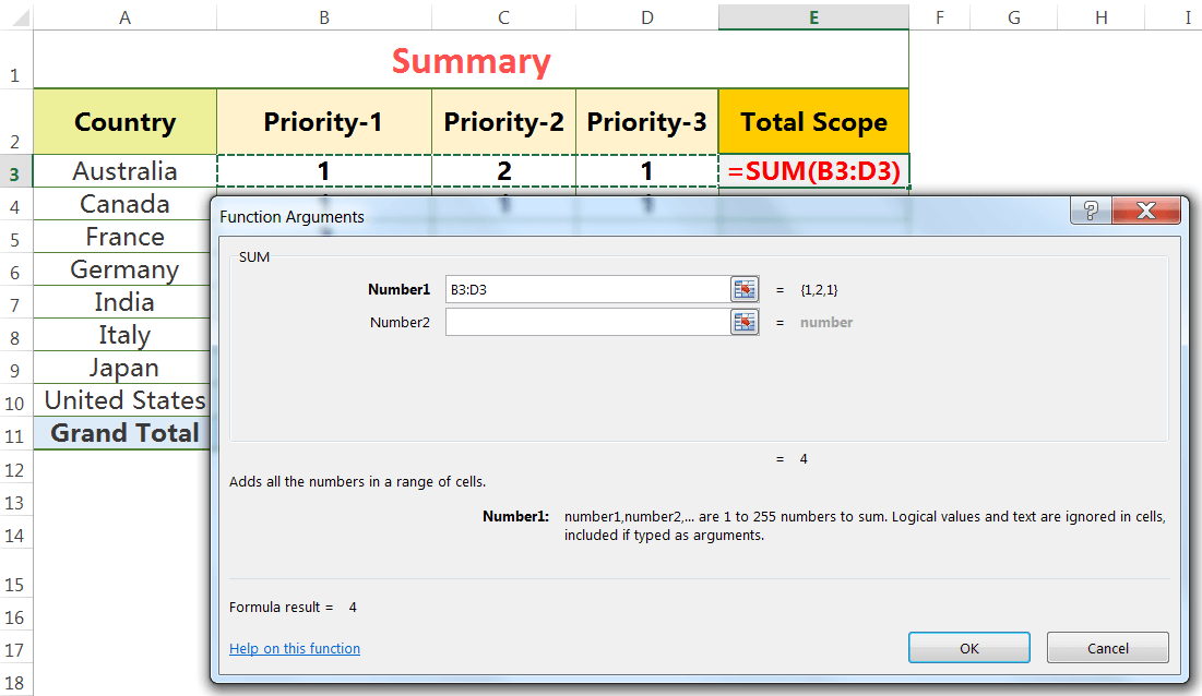
(03) As a result, the ‘Function Arguments’ dialog box appears. Depending on the individual function’s arguments, select the required cells for each argument expected by the function. We can select a cell or range of cells and Excel automatically adds the references to the argument. However, we can also type a range or cell address directly in the argument text box.
Selects the range (i.e., B3:D3) in the Number1 box. If required, we can select multiple necessary cell references to complete all of the function’s arguments.
(04) When finished constructing the arguments, press Enter or click OK to accept the formula.
Note: Excel displays the function results in the cell and the function appears in the Formula bar.
• Method 3: Apply SUM Function With ‘Insert Function’ button on the Formula Bar
(01) Select the cell where to apply the SUM function.
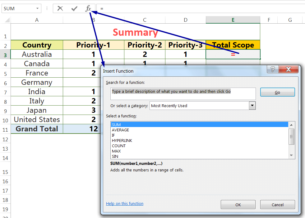
(02) Click the ‘Insert Function’ button (fx) on the formula bar which will open the ‘Insert Function’ dialog box. Excel automatically place an equal sign (=) in the cell.
Either type and search SUM function in the ‘Search for a function:’ box or click to choose a category from ‘Or select a category:’ drop-down list and select the SUM function ➪ then click OK.
➢ Alternatively, go to the ‘Formulas’ tab ➪ Click the ‘Insert Function’ button (fx) in the function library group.
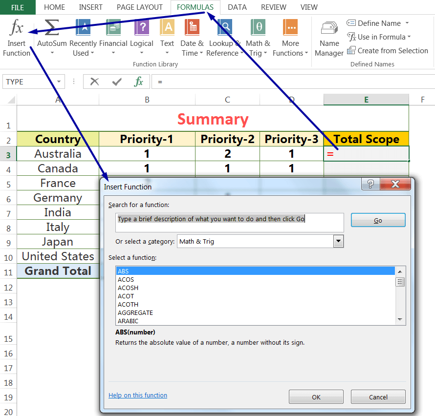
(03) As a result, another ‘Function Arguments’ dialog box opens ➪ Select the range (i.e., B3:D3) in the Number1 box; similarly we can select multiple different ranges ➪ Press Enter or click OK to accept the formula.
• Method 4: Apply SUM Function With AutoSum Excel
When we apply AutoSum, Excel first checks is there any contiguous range of values above the current cell, if there are, Excel will sum the values above it; otherwise, it will check are there any values to the left of it and if there are it will sum those values. We can change the range if required.
02. HOW TO USE AUTOSUM IN EXCEL?
We can apply the AutoSum Excel function in 03 ways:
➢ Method 1: Excel AutoSum Shortcut (Alt+=)
(01) Click a cell beneath a contiguous range or a cell right in the contiguous range where we want to insert a sum total.
(02) Press Alt + = which will apply the AutoSum in Excel and by default select the suggested range (or drag to select the desired range).
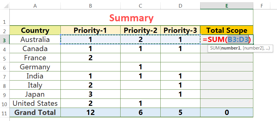
(03) Finally, press the Enter key to accept the formula.

➢ Method 2: AutoSum Excel by clicking the AutoSum Button on the ‘HOME’ tab
(01) Click a cell beneath a contiguous range or a cell right in the contiguous range where we want to insert a sum total.
(02) Go to the Home tab ➪ click the Autosum button in the Editing group. As a result, Excel by default selects the suggested range (or, drag to select the desired range).

(03) Press the Enter key to accept the formula.
➢ Method 3: AutoSum Excel by clicking the AutoSum Button on the ‘FORMULAS’ tab
(01) Click a cell beneath a contiguous range or a cell right in the contiguous range where we want to insert a sum total.
(02) Go to the Formulas tab ➪ click the Autosum button in the Function Library group. Similarly, Excel by default selects the suggested range (or, drag to select the desired range).

(03) Press the Enter key to accept the formula.
03. HOW TO EXCEL AUTOSUM HANDLING BLANK CELLS IN A RANGE?
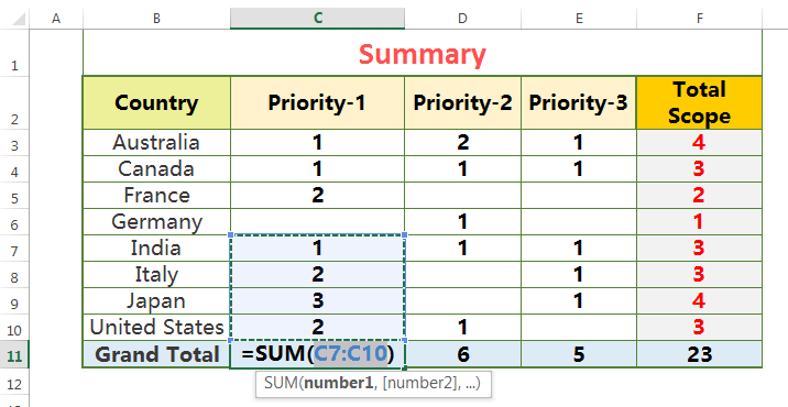
Excel AutoSum does not include any cells in its range after reaching a blank cell. In this case, we can change the range manually in two ways:
(i) First select the range in the SUM() function and extend the range by Shift and Navigation keys. After the selection of the new range, press Enter to accept the change in the formula.
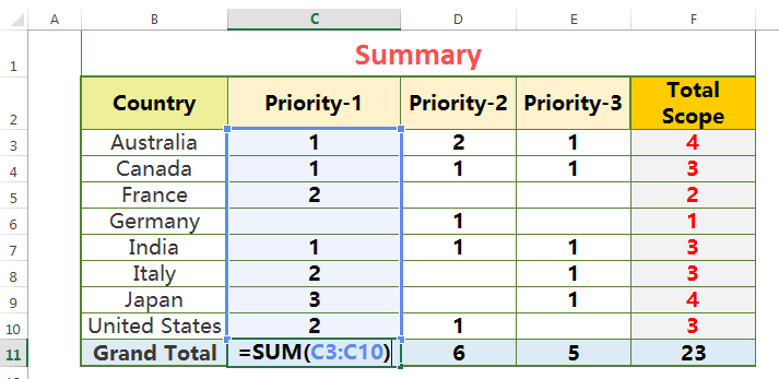
(ii) Another way to extend the range by dragging one of the fill handles of the selected range and extend the range so that it includes all the cells we want. Finally, press Enter to accept the change in the formula.


Premium Courses on ed2go
Premium Courses on Coursera
Premium Courses on FutureLearn Limited
Premium Courses on Udemy

30+ BEST ADVANCE EXCEL COURSES | By Coursera, Udemy |
36+ BEST ADVANCED EXCEL COURSE ONLINE | By ed2go |
80+ Excel Shortcuts with ALT Key || Best Hotkey of Keyboard Shortcuts
10 Examples of Text to Columns || How to Split Cells/Columns in Excel
04 Best Ways: How to Transpose Data in Excel
How to use VLOOKUP Function in Excel || Must know Do OR Dont’s ||
03 Best Ways: Excel REVERSE VLOOKUP | VLOOKUP to the left |
03 Best Ways: EXCEL DOUBLE VLOOKUP/ IFERROR VLOOKUP/ NESTED VLOOKUP
Thanks for your interest joining to Advance Excel Forum community.
Something went wrong.

Join Our Community List
Subscribe to our mailing list and get interesting stuff and updates to your email inbox.
* VERIFY & CONFIRM YOUR EMAIL * We respect your privacy and take protecting it seriously*.


