(I) WHAT IS PASTE SPECIAL IN EXCEL?

Paste Special in Excel provides a more powerful advanced pasting feature with a number of pasting options, such as cell content, formulas, values, formatting, and much more. The Excel Paste Special feature only works with the Copy command (Ctrl+C) but it wouldn’t work after using the Cut commands (Ctrl+X).  

The Paste Special command is often used to perform the following types of operations:

➢ Paste only the values in cells (not the formulas and formatting) to a different part of a worksheet.

➢ Paste only the formulas in cells (not the formatting) to a different part of a worksheet.

➢ Transpose data in columns to rows and vice versa.

➢ Transform a range of numbers by adding, subtracting, dividing, or multiplying each number in the range by a given constant.

• How to Apply Paste Special in Excel? 

➢ Method 1: Using Excel Paste Special Shortcut

Select the cell or range of cells ➪ Copy them (Ctrl+C) ➪ Press Excel shortcut Alt+E+S (press sequentially Alt, E, S) which will open the Paste Special dialog box. 

➢ Method 2: Using Alternative Excel Paste Special Shortcut 

Alternatively, select the cell or range of cells ➪ Copy them (Ctrl+C) ➪ Press Excel shortcut Alt+Ctrl+V which allows us to open the Paste Special dialog box. 

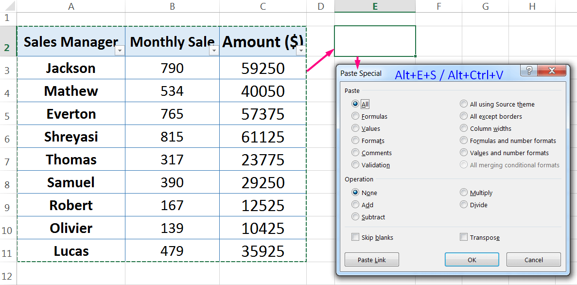
➢ Method 3: Using the Ribbon

Alternatively, select the cell or range of cells ➪ Copy them (Ctrl+C) ➪ Go to the ‘Home‘ tab ➪ Click on ‘Paste‘ drop-down arrow ➪ Select ‘Paste Special’ option.

➢ Method 4: Using Right Click Option  

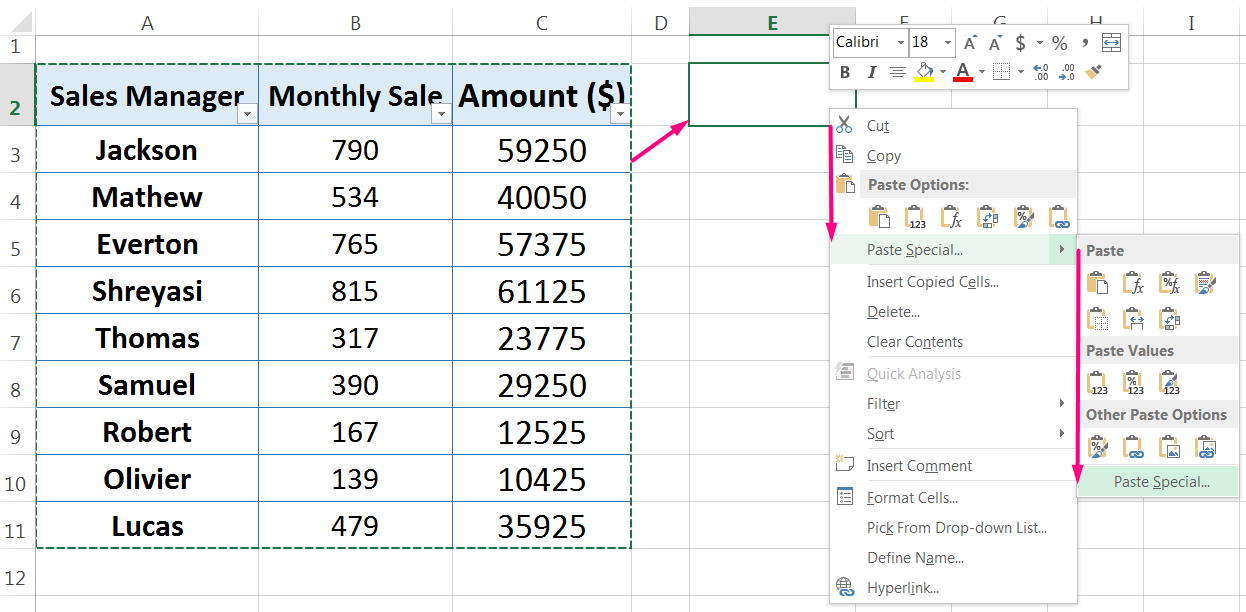
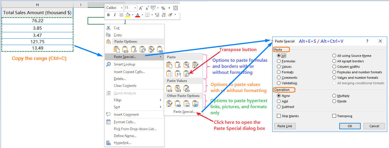
Alternatively, select the cell or range of cells ➪ Copy them (Ctrl+C) ➪ right-click on any selected cell ➪ choose the ‘Paste Special…‘ command under the Paste Options.

(II) WHAT IS BREAK LINKS IN EXCEL?

Whereas, Break Link in Excel severs the ties with the linked workbook. Excel replaces any linked formulas with the most recent data. If we have external references in a workbook and we have no longer need the links, then we can convert the external reference formulas to values, thereby severing the links with the help of break link.

• How to Break Links in Excel? 

➢ Method 1: Using Break Links in Excel Shortcut

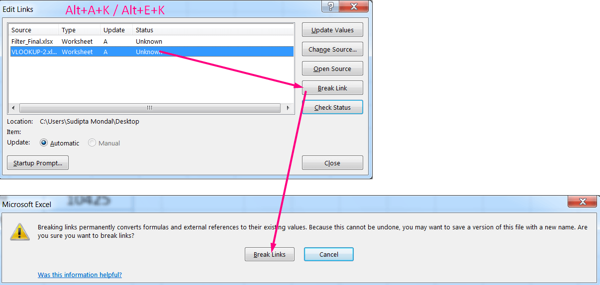
Place cursor anywhere in the worksheet ➪ Press Excel shortcut Alt+A+K (sequentially press Alt, A, K) which will open the Edit Links dialog box ➪ Select the linked file in the list, and then click Break Link.

➢ Method 2: Alternate Using of Break Links in Excel Shortcut

Alternatively, place the cursor anywhere in the worksheet ➪ Press Excel shortcut Alt+E+K (sequentially press Alt, E, K) which will open the Edit Links dialog box ➪ Select the linked file in the list, and then click Break Link.

➢ Method 3: Using the Ribbon

Alternatively, we can access the Edit Links dialog box using the ribbon. Go to the ‘Data‘ tab  ➪ Select the ‘Edit Links‘ in the Connections group, select the linked file in the list, and then click Break Link.

Break Links generally break all the external links (i.e., VLOOKUP, HLOOKUP formulas are often used to retrieve values from the other workbooks).

To do the same work (converting formulas to values), Break Link works faster than Paste Special in Excel. At a glance, we should know the features and differences between them:

(III) ADVANTAGES OF PASTE SPECIAL IN EXCEL:

There are a number of advantages to using the Paste Special in Excel: 

➢ Paste ‘All‘ is a straightforward paste, identical to Home ➪ Clipboard ➪ Paste (Ctrl+V).

➢ The Paste Special → ‘Values‘ and ‘Values and number formats‘ options are very often used to convert any formulas to values.

➢ The Paste Special → ‘Formulas‘ and ‘Formulas and number formats‘ options are very helpful when we want to copy the formula from source data, but do not want the associated cell formatting. 

➢ The Paste Special → ‘Formats‘ option allows users to copy cell formatting only. 

➢ The Paste Special → ‘Comments‘ copy cell notes from one cell to another but does not disturb the actual contents of the cell. 

➢ The Paste Special → ‘Validation‘ copy the validation criteria. 

➢ The Paste Special → ‘All except borders‘ option is a handy feature to ensure that the borders of the new range aren’t disturbed when new data or formulas are copied over the cells. 

➢ Perform a mathematical operation using the contents of the copied cells with the pasted cell contents.

➢ The Paste Special → ‘Skip blanks‘ option ignores blank cells.

➢ The Paste Special → ‘Transpose‘ option allows users to arrange a copied data in such a way where row data become column data and column data become row data.

➢ Link the pasted cells to the copied cells.

(IV) SUMMARY OF EXCEL PASTE SPECIAL OPTIONS AND THEIR APPLICATIONS

Note: Depending upon the content we are copying and the ‘Paste’ options that we have selected, some options may be unavailable.  

Note: Note Mathematical operations can only be applied to values. If we performing one of the mathematical operations (Add, Subtract, Multiply, or Divide) must select either All, All except borders, or Values and number formats from the Paste options.

(V) HOW TO USE PASTE SPECIAL IN EXCEL?

A. Using Paste Special in Excel to Perform Advanced Pasting

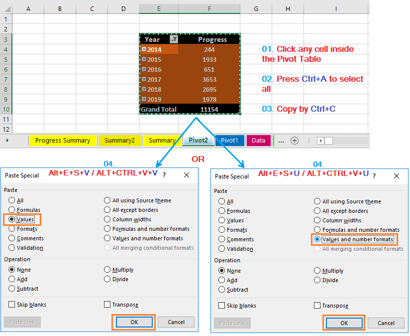
(01) Converting Formulas and Pivot table into ‘Values’

We can paste formulas or pivot tables with their values in two ways, but in both cases, we select the range or the entire database.  

➢ Values: Select the range(s) ➪ Copy (Ctrl+C) ➪ use Excel Shortcut Alt+E+S+V or Alt+Ctrl+V+V ➪ press Enter or click OK.

➢ Values and number formats: Select the range(s) ➪ Copy (Ctrl+C) ➪ use Excel Shortcut Alt+E+S+U or Alt+Ctrl+V+U ➪ press Enter or click OK. 

(02) Pasting All the ‘Formulas’ of the Copied Range at Another Location

Pastes the formulas used in the copied cells or ranges in two ways: 

➢ Formulas: Select the range(s) ➪ Copy (Ctrl+C) ➪ use Excel Shortcut Alt+E+S+F or Alt+Ctrl+V+F to select the ‘Formulas’ option ➪ press Enter or click OK. 

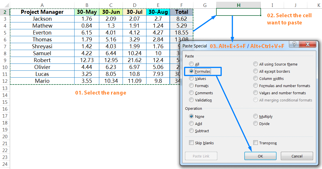
➢ Formulas and number formats: This option is mostly used rather than the ‘Formulas’ option. This option is the same as Formulas, except that it retains the formatting for any numbers you copy. So Excel will retain currency signs ($), percentage signs (%), and thousands of separators in numbers, but it drops the formatting for fancy fonts, colors, and borders.

Select the range(s) ➪ Copy (Ctrl+C) ➪ use Excel Shortcut Alt+E+S+R or Alt+Ctrl+V+R to select the ‘Formats’ option ➪ press Enter or click OK. 

(03) Pasting Similar ‘Formatting’ of the Copied Range

Pastes only the formatting of the copied data, but not the data.

Select the range(s) ➪ Copy (Ctrl+C) ➪ use Excel Shortcut Alt+E+S+T or Alt+Ctrl+V+T to select the ‘Formats’ option ➪ press Enter or click OK. 

(04) Pasting Similar ‘Column Widths’ of the Copied Range

Pastes the column widths so they match the width of the columns of the copied cells.

Select the range(s) ➪ Copy (Ctrl+C) ➪ use Excel Shortcut Alt+E+S+W or Alt+Ctrl+V+W  to select the ‘Column widths’ option ➪ press Enter or click OK. 

(05) Pasting All ‘Comments’ to the entire Range

Pastes only comment attached to the cell.

➢ Example 1: In the given example, Cell A3 has a comment and we want to copy that entire ranges instead of typing comments in each cell.   

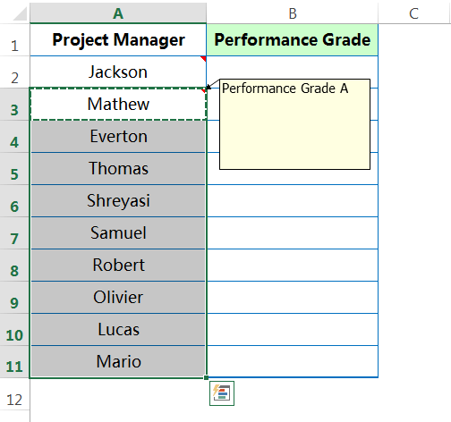
Copy (Ctrl+C) the cell A3 with the comment ➪ then select the area want to paste the comments ➪ use Excel shortcut Alt+E+S+C / Alt+Ctrl+V+C to select the ‘Comments’ option ➪ then press Enter or click OK.  

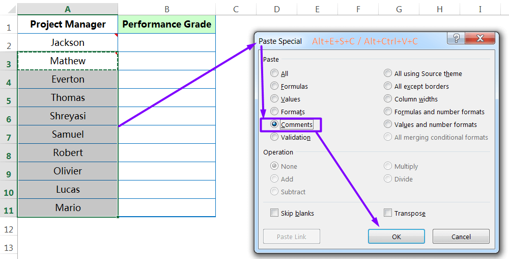
Entire selected area copied with the same comments. 

➢ Example 2: Similarly, we can copy all the comments sequentially from a range into the other range. 

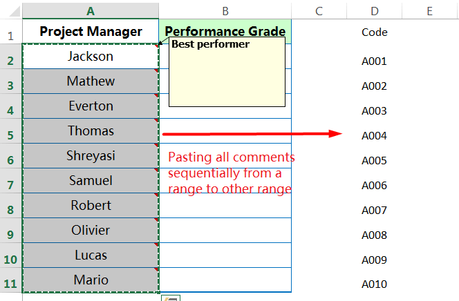
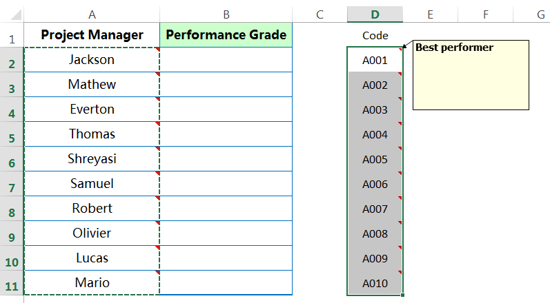
Select the entire range (i.e., A2:A11) with comments ➪ copy the range by Ctrl+C ➪ either select the first cell or select the entire range of the pasted range ➪ press Alt+E+S+C / Alt+Ctrl+V+C to select the ‘Comments‘ option ➪ press Enter or OK.

All the comments copied sequentially from one range to the other range successfully.  

(06) Pasting ‘Validation’ rules in the Entire Range

Pastes data validation rules of a copied cell to the entire range(s).

➢ The First Step to Apply a Data Validation in a Cell:

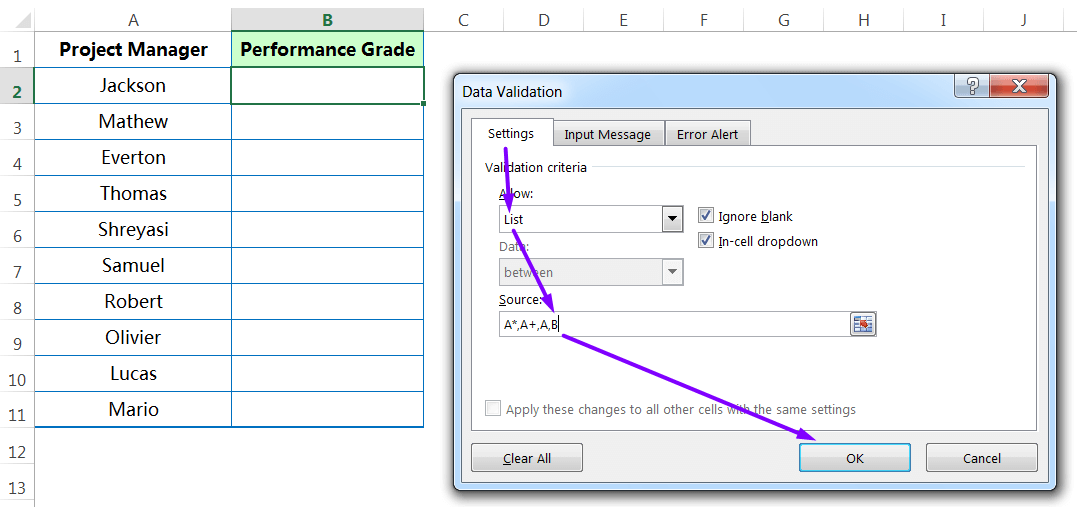
Select a cell wanted to apply Data validation ➪ press Alt+D+L to open the Data Validation dialog box.

Go to the Settings tab ➪  click on the ‘Allow’ drop-down list ➪ select ‘List’ ➪ in the box, type the criteria with a comma separator ➪ press Enter or click OK.

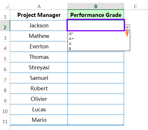
Data Validation is applied and ready to use.  

➢ The Second Step to Apply Data Validation Rules in the Entire Ranges:

Copy the cell where Data Validation rules applied ➪ then select the range of cells wanted to apply the validation ➪ press Excel shortcut Alt+E+S+N or Alt+Ctrl+V+N to select the ‘Validation’ option under the Paste Special dialog box ➪ press Enter or click OK.

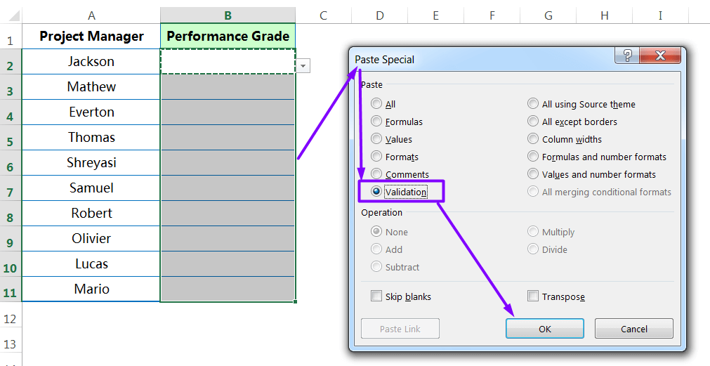
Data Validation is applied in the selected range. 

B. Using Paste Special in Excel to Perform “Calculations”

Paste Special can perform calculations while pasting. Paste Special has operation options for Add, Subtract, Multiply, and Divide. A single cell value can be pasted to a group of cells while performing an arithmetic operation, or a group of cells can be pasted to another group of cells while performing an arithmetic operation.

(01) Adding Similar Value in the Range

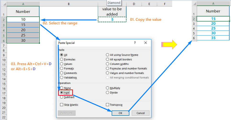
Now, we want to add the value 5 in cell C2 to each of the cells in the range A2:A6. Figure 1

We would perform the following steps:

• Select cell C2 and then make a copy.

• Select the cells where we want to paste the operation. In this case that would be range A2:A6.

• Press Alt+E+S+D / Alt+Ctrl+V+D to select the Add operation under the Paste Special dialog box

(Alternatively, Right-click one of the selected cells ➪ then select Paste Special ➪ Select the Add operation). As a result, value 5 has been added to each value in the pasted range.

(02) Adding Different Values in the Range

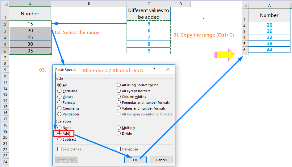
We can combine a group or multiple groups while performing an arithmetic operation. If we wanted to add the different values present in range C2:C6 to the individual values in range A2:A6, as shown in Figure 2, we would perform the following steps:

• Select the cell range C2:C6 and then make a copy.

• Press Alt+E+S+D / Alt+Ctrl+V+D  to select the ‘Add’ operation under the Paste Special dialog box.

(Alternatively, Right-click one of the selected cells a then select Paste Special ➪ Select the Add operation).

(03) Adding Few Values in the Range

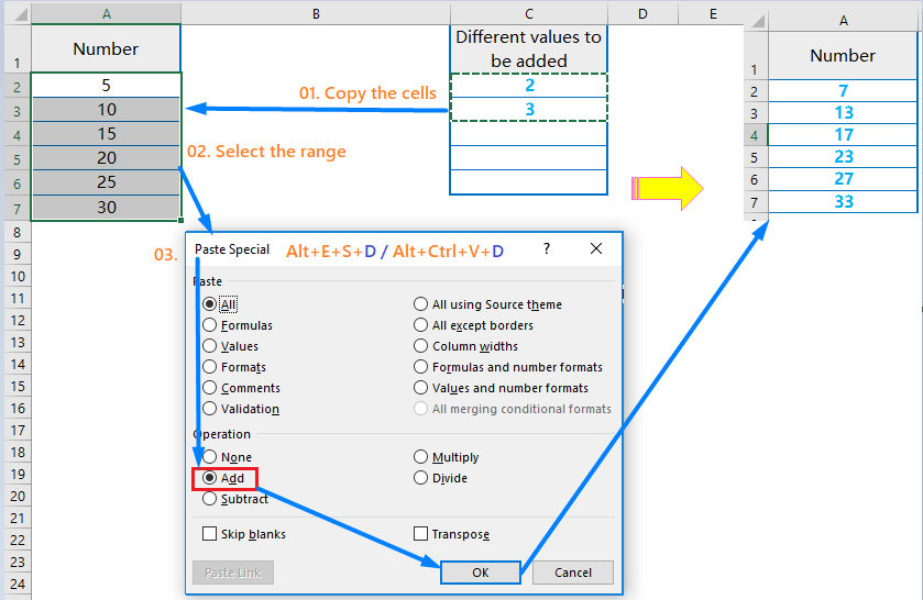
If we were copying fewer values than we were pasting, then the copied values would repeat their pattern. The value in cell C2 would be added to the value in cell A2. The value in cell C3 would be added to the value in A3. Then the value in cell C2 would be added to the value in A4, and the value in C3 would be added to the value in A5.

(04) Multiplying a Value in the Range

If we want to increase the sales target price of every Project Managers by 15%, then we use the Multiply option of Paste Special in Excel. Remember that after increasing 15%, we get an increased value of 115. That means if we multiply 1.15% in the range, we get the actual increased value.    

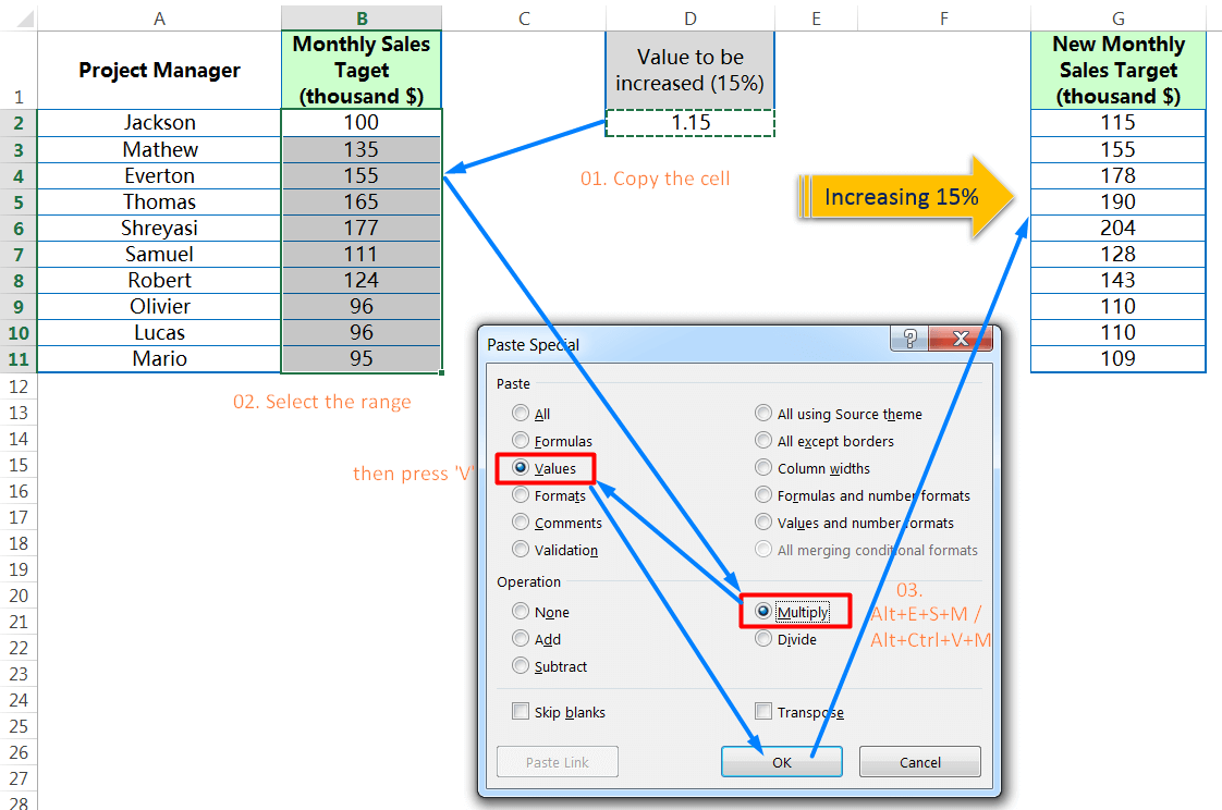
• Copy cell D2 contains an increased percentage value, i.e., 1.15% by pressing Ctrl + C.

• Select cell range B2:B11.

• Press Excel shortcut Alt+E+S+M / Alt+Ctrl+V+M to select the ‘Multiply‘ option under the Paste Special dialog box. After that press only V or U to select the ‘Values‘ or ‘Values and number formats‘, respectively. 

• Press Enter or click OK to get the increased value.

(C) Using Paste Special in Excel to Avoid “Skip Blanks”

When we copy a range of cells, any cells that are blank in the copied range will overwrite any cells in the pasted range, thus making those cells also blank.

However, if we use the Skip Blanks option of Paste Special in Excel, the blank cells in the copied range will not overwrite the data in the cells in the pasted range.

• Copy cell range D2:D11 with the blank cells by pressing Ctrl + C.

• Select cell range B2:B11.

• Press Excel shortcut Alt+E+S+B /Alt+Ctrl+V+B to select the ‘Skip blanks‘ option under the Paste Special dialog box. After that press only V or U to select the ‘Values‘ or ‘Values and number formats‘, respectively. 

• Press Enter or click OK to get the result. 

(D) Using Paste Special in Excel to ‘Transpose’ Rows and Columns

The Paste Special command has a ‘Transpose‘ option that is used for converting row data to column data and vice versa.

We would like to use the Transpose function when the row headings require to arrange as the column headings and the column headings as the row headings. Rather than manually retyping the headings, we can easily flip-flop them by using Paste Special’s Transpose option.

Select the range ➪ copy (Ctrl+C) ➪ press Alt+E+S+E or Alt+Ctrl+V+E to select the ‘Transpose’ option ➪ simultaneously, press ‘R’ from the keyboard to select the ‘Formula and number formats’ ➪ press Enter or click OK.

Finally, the dataset is transposed!

Note: You should learn 04 ways to apply transposed data in Excel.

(VI) HOW TO APPLY BREAK LINK IN EXCEL?

(A) How to Manage Linked Workbooks

As we work with a linked workbook, we might need to replace a source file or change where we stored the source and destination files. However, replacing or moving a file can affect the linked workbook. Keep in mind the following guidelines to manage our linked workbooks:

➢ If we rename a source file, the destination workbook won’t be able to find it. A dialog box opens, indicating “This workbook contains one or more links that cannot be updated.” Click the Continue button to open the workbook with the most recent values, or click the Change Source button in the Edit Links dialog box to specify the new name of that linked source file.

➢ If we move a source file to a different folder, the link breaks between the destination and source files. Click the Change Source button in the Edit Links dialog box to specify the new location of the linked workbook.

➢ If we receive a replacement source file, we can swap the original source file with the replacement file. No additional changes are needed.

➢ If we receive a destination workbook, but the source files are not included, Excel will not be able to find the source files, and a dialog box opens with the message “This workbook contains one or more links that cannot be updated.” Click the Continue button to open the workbook with the most recent values, or click the Break Link button in the Edit Links dialog box to replace the external references with the existing values.

➢ If we change the name of a destination file, we can open that renamed version destination file without affecting the source files or the original destination file.

(B) Updating Linked Workbooks

➢ When the workbooks are linked, it is important that the data in the destination file accurately reflect the contents of the source file. When data in a source file changes, we want the destination file to reflect those changes.

➢ If both the source and destination files are open when we make a change, the destination file is updated automatically.

➢ If the destination file is closed when we make a change in a source file, we choose whether to update the link to display the current values or continue to display the older values from the destination file when we open the destination file.

(C) To Convert all External Reference Formulas into Values

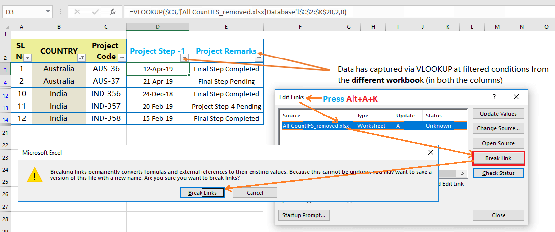
➢ Go to the ‘Data’ tab ➪ Click on the ‘Edit Links’ command ➪ an ‘Edit Links dialog’ box opens ➪ click the Break Link button. Alternatively, press the Excel shortcut Alt+A+K to open the Edit Links dialog box and then press Alt+B to click the Break Link button (figure below Example 2).

➢ A dialog box opens, Break Link alerts us that breaking links in the workbook permanently convert formulas and external references to their existing values.

➢ Click the Break Links button. No links appear in the Edit Links dialog box.

➢ Click the Close button.

(VII) BEST USES OF BREAK LINKS INSTEAD OF PASTE SPECIAL IN EXCEL

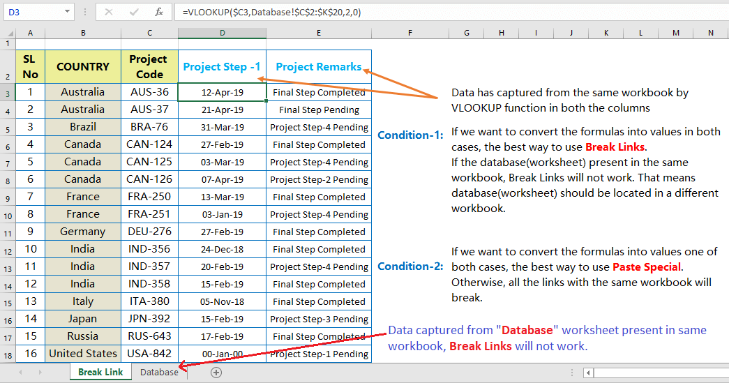
(01) Example 1: While Database ties with the external links (or external reference formulas) of the same or different worksheets in the same workbook and we want to break all the links – ‘Excel Break Links‘ is the best way to sever the links. 

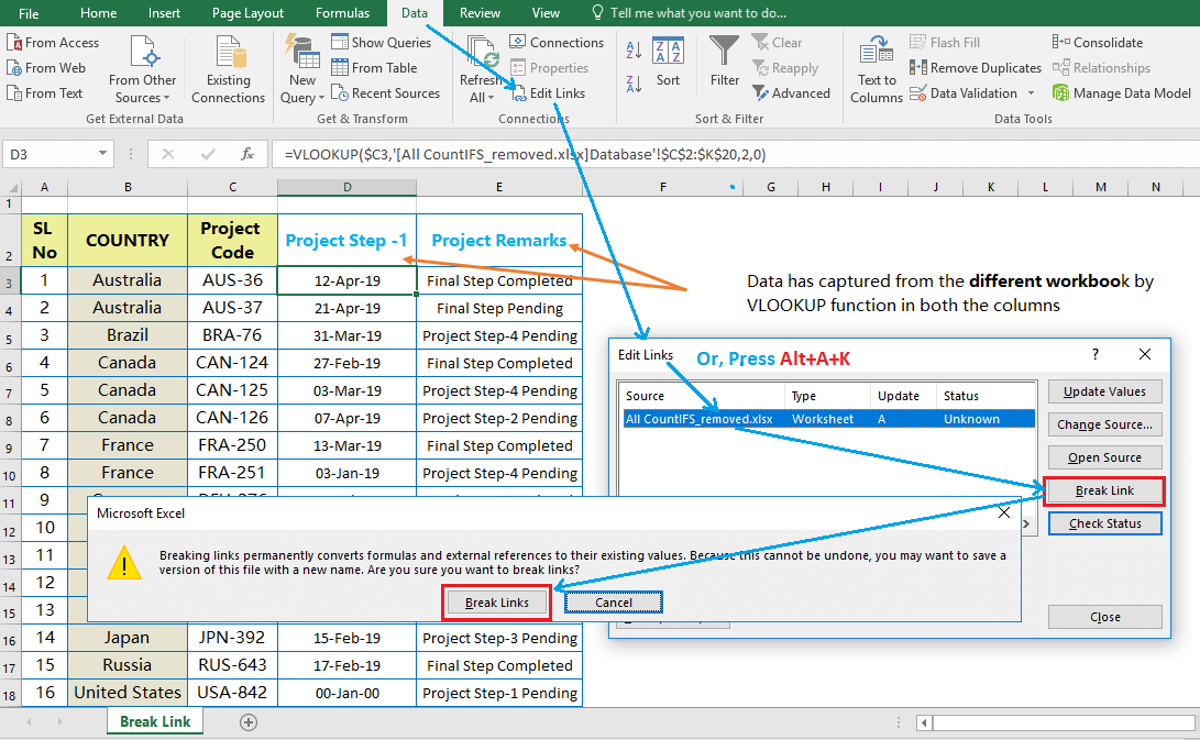
(02) Example 2: While the VLOOKUP and/or the HLOOKUP functions are applied to retrieve values from other sources in a filtered Dataset and we want to break all the Links without removing the filter – the Excel Break link is the only solution to break all the links and convert formulas to their values in the filtered dataset. 

Step 1:

(VIII) COMPARISON BETWEEN PASTE SPECIAL AND BREAK LINK IN EXCEL