TABLE OF CONTENTS:
Toggle(01) UNDERSTANDING EXCEL WORKSHEET STRUCTURE
Data we type into Excel worksheet is commonly known as Excel sheet. Whether we use a single worksheet or a large collection of sheets, every worksheet is structured in the same way.
➢ COLUMNS AND ROWS:
Excel Worksheets are formatted as a grid formed by columns and rows. Each worksheet has 16,384 columns (the last column is XFD) and 1,048,576 rows. Every column and row has a unique identifier. Columns are labelled by letters arranged alphabetically, and rows are labelled by number, so the first cell address in a worksheet is identified as A1.
➢ CELLS AND CELL ADDRESSES:
Every intersection of a column and a row creates a cell. Cells are the receptacles for Excel data. In an Excel worksheet, every cell has a unique name is called cell address or cell references. Cell names consist of the column and row number, with the column always listed first. For example, cell A1 is the first cell in the worksheet. The next cell to the right is B1.
Active Cell: The active cell in a worksheet is always surrounded by a highlighted border, called the selector. The Name box is located on the far left side of the Formula bar, which always displays the name of the current cell.
Cell Ranges: While working with data in an Excel worksheet, we can group related data into a range. A range is simply a group of related cells that we can connect. By grouping cells in a range, we can apply formatting, or printing to the entire collection, or move or copy the range data at once to another location. Additionally, ranges are particularly useful when we try to create a formula that references to groups of cells.
Worksheet Tabs: By default, every Excel workbook starts out with a single worksheet (i.e., Sheet1). Each worksheet is identified by a tab at the bottom of the sheet. The active worksheet always appears at the top of the stack. We can add more worksheets as per requirement using the Insert Worksheet tab (+ sign) to the right of the Sheet1 tab. We can also give our worksheets unique names to better identify their content.
Creating a multiple-worksheets workbook takes some planning and maintenance. Worksheet tab names should reflect the contents of the respective worksheets, for example Summary, Master Data etc. In addition, we can insert, copy, move, and delete Excel worksheets within a workbook.
(02) HOW TO ADD EXCEL WORKSHEETS INTO A WORKBOOK?
By default, a new workbook includes only one worksheet. Sometimes we need more than one worksheet in the workbook. We can add blank worksheets to an Excel workbook any of the following methods: ➢ Using Excel Shortcut: Shift+F11 (a new Excel worksheet added before the active sheet tab). ➢ Using the Mouse Right-Click: Right-click the worksheet tab before which we want to insert a new worksheet ➪ Then click Insert from the shortcut menu ➪ Click Worksheet icon (by default selected) in the Insert dialog box on the General tab ➪ then click OK or press Enter (a new Excel worksheet added before the active sheet tab).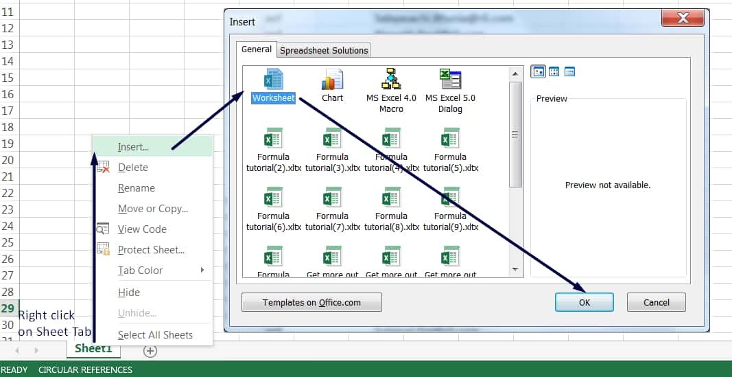 ➢ Using Button: Click the New sheet button which is the plus sign icon located to the right of the last visible sheet tab (a new Excel worksheet is added after the active sheet tab).
 ➢ Using the Ribbon: Go to the Home tab ➪ in the Cells group, click the Insert arrow ➪ Then click Insert Sheet (a new Excel worksheet is added after the active sheet tab).
Equivalently, use the Excel shortcut Alt+H+I+S (sequentially press Alt, H, I, S).

(03) HOW TO RENAME AN EXCEL WORKSHEET TAB?
The default worksheet names such as Sheet1, Sheet2 etc., do not describe the contents of the worksheet. We should rename worksheet tabs to reflect the sheet contents, such as Master Data, Summary etc. Sheet names can contain as many as 31 characters, and spaces are allowed. However, we can’t use the following characters in sheet names:: colon
/ slash
\ backslash
[ ] square brackets
? question mark
* asterisk
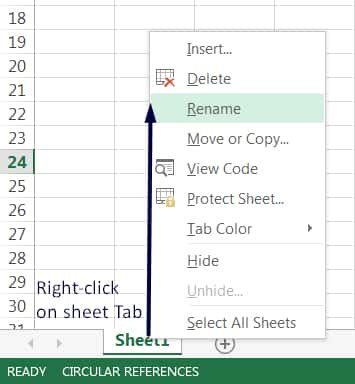
➢ Using the Excel Shortcut: Use the Excel shortcut Alt+O+H+R (sequentially press Alt, O, H, R) or Alt+H+O+R (sequentially press Alt, H, O, R) which will highlight the sheet name for editing ➪ Type a new name ➪ Press Enter. ➢ Using the Mouse Double-click: Double-click a sheet tab will put the tab text in edit mode ➪ Type a new name ➪ Press Enter. ➢ Using the Mouse Right-click: Right-click a sheet tab ➪ Select Rename from the shortcut menu ➪ Type a new sheet name ➪ Finally press Enter.
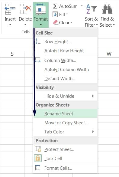
 ➢ Using the Ribbon: Open the worksheet/tab we want to rename ➪ Go to the Home tab ➪ Click Format in the Cells group ➪ Select Rename Sheet ➪ Type a new sheet name ➪ Press Enter.
(04) HOW TO CHANGE THE EXCEL WORKSHEET TAB COLOR?
We can change the color of each worksheet tab to emphasize the difference between the sheets and users can easily distinguish them. ➢ Using the Excel Shortcut: Alt+O+H+T (sequentially press Alt, O, H, T) OR Alt+H+O+T (sequentially press Alt, H, O, T) ➢ Using the Mouse Right-Click: Right-click a sheet tab ➪ Select ‘Tab Color’ from the shortcut menu ➪ Select a color from the color palette ➪ finally press Enter.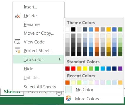 ➢ Using the Ribbon: Open the worksheet/tab we want to rename ➪ Go to Home tab ➪ Click Format in the Cells group ➪ Select Tab Color from Organize Sheets section ➪ Select a theme color from the color palette ➪ Finally press Enter.
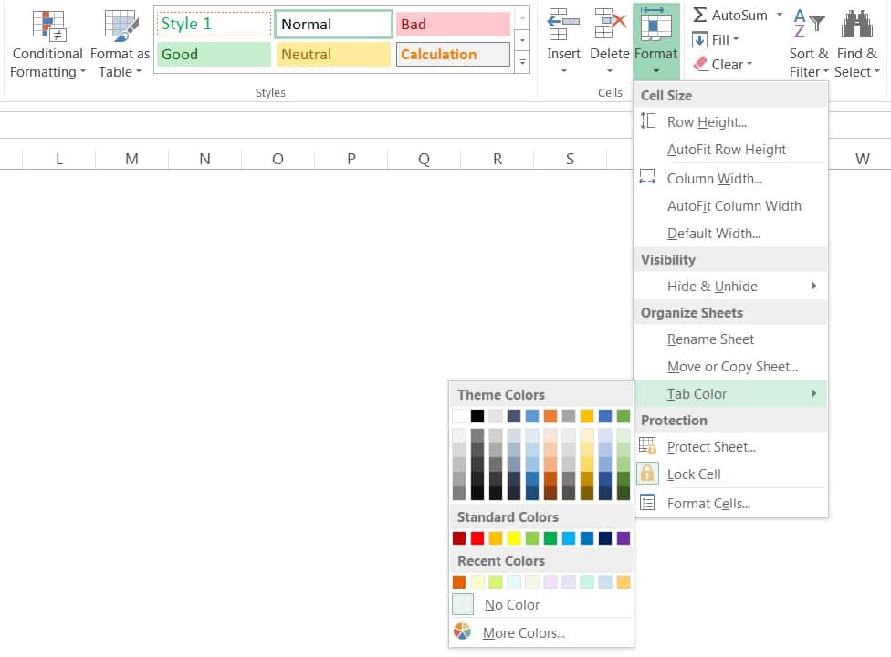 Note: After applying tab color, the color is visible only when the Excel worksheet is not the active sheet.
(05) HOW TO COPY A SHEET IN EXCEL?
OR, HOW TO DUPLICATE A SHEET IN EXCEL?
Copying the entire worksheet saves a lot of valuable time in entering and formatting the new worksheet, and it preserves the column widths and row heights. We can move or copy the worksheet(s) to another existing workbook or the same workbook with the help of the ‘Move or Copy’ dialog box. In case of multiple worksheets, select them and make a group by pressing and holding down the Ctrl key.➢ METHOD 1: USING ‘MOVE OR COPY’ DIALOG BOX
(A) TO OPEN THE ‘MOVE OR COPY’ DIALOG BOX We can follow any of the following 4 methods to open the ‘Move or Copy’ dialog box: • Using the Excel Shortcut: Press Alt+E+M (sequentially press Alt, E, M). • Using the Excel Shortcut: Press Alt+H+O+M (sequentially press Alt, H, O, M) • Using Mouse Right-Click: Right-click the worksheet tab ➪ Then click ‘Move or Copy’.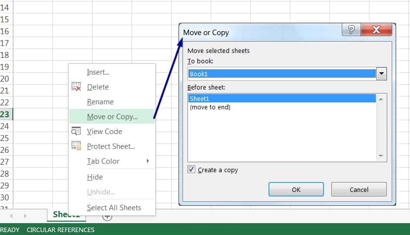 • Using the Ribbon: Go to the Home tab ➪ Click Format drop-down under Cells group ➪ Then click ‘Move or Copy Sheet…’ in the Organize Sheets section,
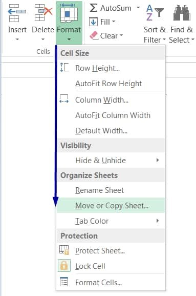 (B) TO MOVE OR COPY AN EXCEL WORKSHEET IN THE SAME WORKBOOK / TO ANOTHER EXISTING WORKBOOK / TO A NEW WORKBOOK
In this case, both the source workbook and destination workbook should be opened. After opening the ‘Move or Copy’ dialog box, do the following:
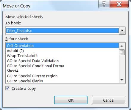 • In the ‘To book’ list, click the destination workbook or create a new workbook.
• In the ‘Before sheet’ box displaying the worksheets of the source workbook, click the worksheet wants to move in the destination workbook.
• Select the ‘Create a copy’ checkbox, otherwise, the source worksheet entirely moves to the destination workbook without a copy.
• Then click OK or press Enter.
➢ METHOD 2: USING ‘DROP & DRAG’
To copy an Excel worksheet, click the worksheet tab, and press the Ctrl key while dragging the tab to its desired location. When we drag, the mouse pointer changes to a small sheet with a plus sign on it. To copy a worksheet in a different workbook, the second workbook must be opened and not maximized. Note: We can move or copy multiple sheets simultaneously. First, select the sheets by clicking their sheet tabs while holding down the Ctrl key. Then, we can move or copy the set of sheets by holding down the Ctrl key. If we move or copy a worksheet in a workbook that already has a sheet with the same name, Excel by default changes the name to make it unique. For example, Sheet1 becomes Sheet1 (2). However, we probably want to rename the copied sheet to give it a more meaningful name. When we move or copy a worksheet in a different workbook, any defined names and custom formats also are copied to the new workbook.(06) HOW TO DELETE A SHEET IN EXCEL?
If we no longer need the data in a worksheet or if we want to get rid of an empty worksheet in a workbook, delete the Excel worksheet. After eliminating extra data or worksheets in a file (workbook), it reduces file size a lot. We can follow any of the following methods: ➢ Using the Excel Shortcut: Either apply the Excel Shortcut Alt+E+L (sequentially press Alt, E, L) or apply Alt+H+D+S (sequentially press Alt, H, D, S). ➢ Using the Mouse Right-Click: Right-click on a sheet tab or group of tabs ➪ Select ‘Delete’ from the shortcut menu.
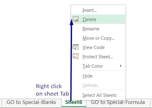 ➢ Using the Ribbon: Select a group of tabs by pressing and holding down the Ctrl key we want to delete ➪ Go to Home tab ➪ click Delete drop-down in the Cells group ➪ select Delete Sheet.
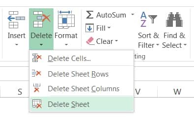 If the sheet(s) we are trying to delete contains data, Excel will display a warning:
Microsoft Excel will permanently delete this sheet. Do you want to continue? Click Delete to delete the worksheet, or click Cancel to keep the worksheet.
Remember that deleting a worksheet from a workbook can’t be undone.
(07) HOW TO REARRANGE EXCEL WORKSHEETS WITHIN A WORKBOOK?
If the workbook includes a Summary worksheet, it should typically be placed at the beginning of the sequence. Additionally, arrange worksheets in chronological order, if possible.
➢ Drag by Mouse: On the tab bar, drag and drop the tab of the Excel worksheet to its desired location. When we drag, the mouse pointer changes to a small sheet, and a small arrow guides us. To move a worksheet to a different workbook, the second workbook must be open and not maximized.

(08) HOW TO GROUP WORKSHEETS IN EXCEL?
➢ GROUP WORKSHEETS IN EXCEL: SELECT THE ADJACENT TABS
We can select multiple adjacent worksheets by clicking the first worksheet tab we want to use and then holding down the Shift key and clicking the last worksheet tab we want to use.
➢ GROUP WORKSHEETS IN EXCEL: SELECT THE NON-ADJACENT TABS
We can select multiple non-adjacent tabs by holding down the Ctrl key and click the tabs we want to use one by one.
(09) HOW TO HIDE & UNHIDE SHEETS IN EXCEL?
In some situations, we may want to hide one or more worksheets. Hiding a sheet may be useful if we don’t want others to see it or modify any formulas or data from the worksheet. When a sheet is hidden, its sheet tab is also hidden. We can’t hide all the sheets in a workbook; at least one sheet must remain visible.➢ HOW TO HIDE SHEETS IN EXCEL?
First, click a Worksheet tab or select a group of tabs we want to hide. • Using the Excel Shortcut: Either apply Alt+O+H+H (sequentially press Alt, O, H, H) or apply Alt+H+O+U+S (sequentially press Alt, H, O, U, S) • Using the Mouse Right-click: Right-click on a sheet tab or group of tabs ➪ Select ‘Hide’ from the shortcut menu.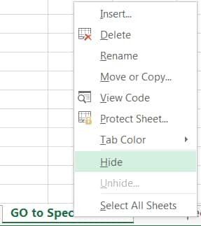 • Using the Ribbon: Open the worksheet/tab or select a group of tabs by pressing and holding the Ctrl key we want to delete ➪ Go to Home tab ➪ Click Format drop-down in the Cells group ➪ Point to Hide & Unhide in the visibility section ➪ select Hide Sheet.
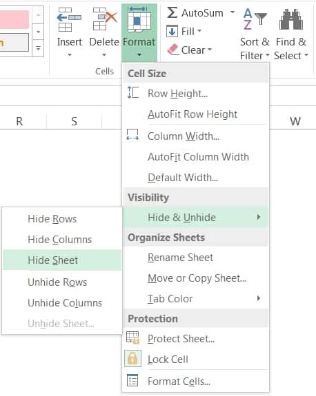
➢ HOW TO UNHIDE SHEETS IN EXCEL?
To unhide a hidden worksheet, we can follow any of the following methods: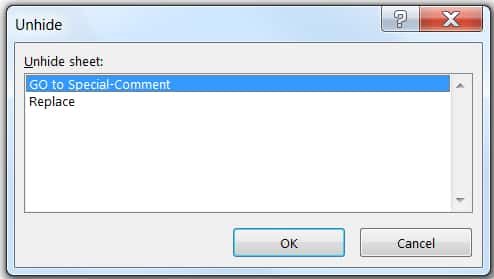 • Using the Excel Shortcut: Either apply Alt+O+H+U (sequentially press Alt, O, H, U) or apply Alt+H+O+U+H (sequentially press Alt, H, O, U, H)
• Using the Mouse Right-click: Right-click any visible sheet tab ➪ Select ‘Unhide’ from the shortcut menu.
• Using the Ribbon: Open any worksheet tab ➪ Go to Home tab ➪ Click Format arrow in the Cells group ➪ Point to Hide & Unhide in the visibility section ➪ select Unhide Sheet.
As a result, Excel opens the Unhide dialog box, which lists all hidden sheets. Choose the sheet that we want to redisplay, and click OK.
We can’t select multiple sheets from this dialog box, so we need to repeat the command for each sheet that we want to unhide. When we unhide a sheet, it appears in its previous position among the sheet tabs.
(10) HOW TO NAVIGATE IN AND AMONG CELLS, WORKSHEETS AND WORKBOOKS?
➢ HOW TO NAVIGATE AMONG CELLS IN AN EXCEL WORKSHEET?
• Using Arrows and Tab Keys: To navigate to a new cell, click it or use the Arrow keys or Tab keys on the keyboard.
• Using Enter: When we press Enter, the next cell down in the same column becomes the active cell.
• Page Up and Page Down Keys: We use the Page Up key to move one screen up and the Page Down key to move one screen down.
• Using Scroll Bars: If we work in a large worksheet, use the vertical and horizontal scroll bars to display another area of the worksheet and click in the desired cell to make it the active cell.
➢ HOW TO NAVIGATE AMONG EXCEL WORKSHEETS?
• Using Excel Shortcut: Ctrl+Page Down: Moving to the next tab (right side). Ctrl+Page Down: Moving to the previous tab (left side). Note: Read usage of CTRL Shortcut Keys • Using Tab Buttons: If there are dots to the left of the worksheet tabs this means that there are more worksheets to the left of those currently showing. These dots are called ellipsis. If there is an ellipsis to the right of the worksheet tabs this means that there are more worksheets to the right of those currently showing.
➢ HOW TO NAVIGATE AMONG EXCEL WORKBOOKS?
• Using Excel Shortcut: Alt+Tab / Ctrl+Tab / Ctrl+F6 – Move to the next workbook Alt+Shift+Tab / Ctrl+Shift+Tab / Ctrl+Shift+F6 – Move to the previous workbook Note: Read usage of Alt Shortcut Keys • Using Left click: Point workbook on the taskbar to open and click it. The keyboard contains several keys that can be used in isolation or in combination with other keys to navigate in a worksheet.| Keystroke | Action |
| ↑ | Move up one cell in the same column. |
| ↓ | Move down one cell in the same column. |
| ← or Shift + Tab | Move left one cell in the same row. |
| → or Tab | Move right one cell in the same row. |
| Home | Move the active cell to column A of the current row. |
| Ctrl + Home | Move to the First cell (A1) of the worksheet. |
| Ctrl + End | Make the rightmost, lowermost active corner of the worksheet—the intersection of the last column and row that contains data—the active cell. Does not move to cell XFD1048576 unless that cell contains data. |
| Page Up | Move the active cell up one screen. |
| Page Down | Move the active cell down one screen. |
| Ctrl + → | Move right to the edge of the nonempty cell in the same row. If there is a blank cell, move right to the first non-blank cell. |
| Ctrl + ← | Move left to the edge of the nonempty cell in the same row. If there is a blank cell, move left to the first non-blank cell. |
| Ctrl + ↑ | Move up to the edge of the nonempty cell in the same column. If there is a blank cell, move up to the first non-blank cell. |
| Ctrl + ↓ | Move down to the edge of the nonempty cell in the same column. If there is a blank cell, move down to the first non-blank cell. |
| Ctrl + Page Up | Move to the previous worksheet |
| Ctrl + Page Down | Move to the next worksheet |
| Ctrl + Shift + Page Up | Select the Current and Next sheet in the workbook |
| Ctrl + Shift + Page Down | Select the Current and Previous sheet in the workbook |
| Alt + Page Up | Move one screen to the left |
| Alt + Page Down | Move one screen to the right |
| Ctrl+G or F5 | Display the Go to dialog box to enter any cell address. |
| Ctrl+F or Shift+F5 | Display the Find dialog box |
| Ctrl+H | Display the Replace dialog box |
| Alt+Tab / Ctrl+Tab / Ctrl+F6 | Move to the next workbook |
| Alt+Shift+Tab/ Ctrl+Shift+Tab/ Ctrl+Shift+F6 | Move to the previous workbook |
| Ctrl+A / Ctrl+Shift+Spacebar | Selects the active data range |
| Ctrl + Spacebar | Selects the entire column |
| Shift + Spacebar | Selects the entire row |
(11) ZOOMING IN OR OUT OF EXCEL WORKSHEET
There are three ways to zoom in/out of the worksheet: ➢ Method 1: We can magnify (zoom in) or shrink (zoom out) the view of the worksheet by using the zoom control button. ➢ Method 2: Press and hold the Ctrl key on the keyboard, at the same time run the mouse wheel to zoom in and out.
➢ Method 3: Go to the View tab ➪ Click Zoom

(12) HOW TO FREEZE PANES IN EXCEL?
Often in large worksheets, it is useful to freeze part of the window and scroll the remaining section of the worksheet. This is particularly true for databases where we want to retain the field or column header on the screen and scroll down through each row or record in the database. It is also important to retain the name in the first column on the screen while we scroll through all the data. To apply the freeze panes go to the View tab ➪ Click Freeze Panes drop-down arrow ➪ Again click Freeze Panes.
However, We had detail explained the Excel Freeze Panes in a separate tutorial and requested you to read the tutorial: 05 Points Should Learn How to Freeze Panes in Excel?
(13) HOW TO FIND AND REPLACE IN EXCEL?
After entering data into the cells of a workbook or worksheet, we can find almost any values, text string, whether it is located in a cell, formula, cell reference, or range name with the help of the Find command in the Find and Replace dialog box. Once it is found, we have the option of replacing the text on a case-by-case basis or all at once using the Replace command in the Find and Replace dialog box. The Excel Find and Replace dialog box includes a feature that allows us to search our worksheet to locate cells that contain specific formatting (for example, a currency symbol). This feature does not locate cells that contain formatting resulting from conditional formatting. ➢ Open Find Dialog Box • Open ‘Find’ Dialog box Using the Excel Shortcut: Click any cell or select the entire range or select the specific cells from where to find the specific value or text ➪ then press Ctrl+F.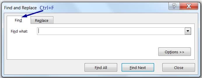 • Open ‘Find’ Dialog box Using the Ribbon: Click any cell or select the entire range or select the specific cells in the worksheet ➪ Go to the Home tab ➪ Click Find & Select drop-down in the Editing group ➪ Click Find.
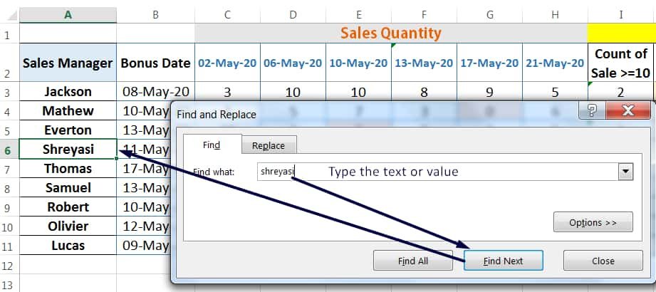
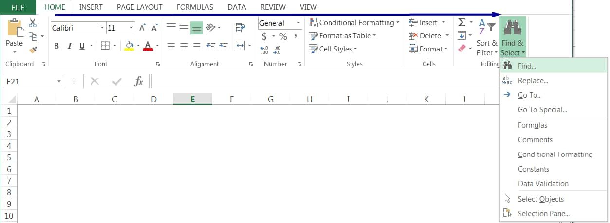 In the Find and Replace dialog box, enter the text string to find under the ‘Find what’ text box ➪ Either click Find All or Find Next ➪ Click Close or press Esc key.
 ➢ Open Replace Dialog Box
• Open ‘Replace‘ Dialog box Using the Excel Shortcut: Click any cell or select the entire range or select the specific cells in the worksheet ➪ then press Ctrl+H.
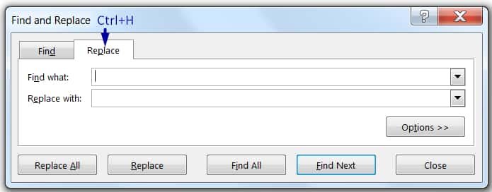 • Open ‘Replace’ Dialog box Using the Ribbon: Click any cell or select the entire range or select the specific cells in the worksheet ➪ Go to the Home tab ➪ Click Find & Select drop-down in the Editing group ➪ Click Find.
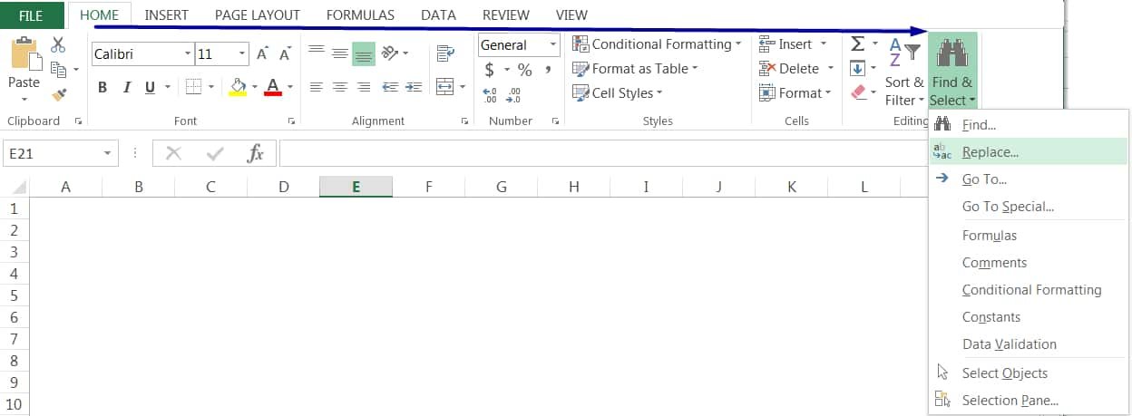 We had detail explained the Find and Replace in Excel in a separate tutorial and requested you to read the tutorial: 07 Points Guided You How to Find And Replace in Excel?
(14) HOW TO USE GO TO SPECIAL IN EXCEL?
When editing a worksheet, Excel Go To Special command is very helpful, but the Excel Go To Special dialog box contains many options to select cells, according to the type of contents they contain.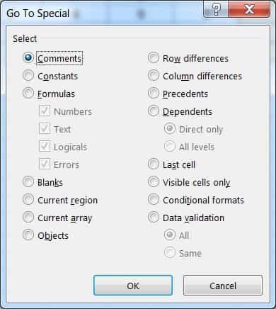
| Option | Description |
| Comments | Selects all cells that contain a comment. |
| Constants | Selects all cells that contain constants (never the formula) of the types specified in one or more of the checkboxes listed under the Formulas option. |
| Formulas | Selects all cells containing formulas that produce results of the types specified in one or more of the following four checkboxes. • Numbers – Selects all cells that contain numbers • Text – Selects all cells that contain text • Logicals – Selects all cells that contain logical values • Errors – Selects all cells that contain errors |
| Blanks | Select the range ➪ Then apply the option, which will select all the cells that are blank. |
| Current region | Select any cell in a range ➪ Then apply the option, which will select the entire dataset. • Equivalently, we press Ctrl+A to select the current region. • Equivalently, we press Ctrl+* (present in number keypad) or Ctrl+Shift+* (above the letter keypad) to select the current region. • Equivalently, Select the heading row by Shift+Spacebar ➪ Move downward with Ctrl+Shift+⬇ |
| Current array | Select any cell in a range ➪ Then apply the option, which will select all the arrays in the data range |
| Objects | Select any cell in a range ➪ Then apply the option, which will select all the objects including the text box |
| Last Cell | Selects the last cell in the worksheet (that is, the lower-right corner) that contains data or formatting. • Equivalently, we press Ctrl+End to move to the last active cell (either contains data or formatting). |
| Visible cells only | Selects only cells that are unhidden. It is helpful to copy the cell references in the filtered cells. |
| Conditional Formats | Selects only cells that contain conditional formatting. • All – Selects all cells that contain conditional formats • Same – Selects all cells that contain similar conditional formats as the current cell |
| Data validation | Selects cells that contain data validation rules. • All – Selects all cells that contain a data validation rule • Same – Selects all cells that contain a similar validation rule as the current cell. |

Premium Courses on ed2go
Premium Courses on Coursera
Premium Courses on Udemy

12 Examples || How to Use Excel Go To Special?
07 Points Guided You How to Find And Replace in Excel?
05 Points Should Learn How to Freeze Panes in Excel?
12 Things Guided You How to Manage An Excel Workbook
03 Useful Methods : Add Numbers With AutoSum Excel
04 Simple to Advanced Methods: How to Filter in Excel?
05 Best Ways: Create Password Protect Excel & Unprotect it
08 Best Examples: How to Use Excel Conditional Formatting?
04 BEST WAYS: HOW TO TRANSPOSE DATA IN EXCEL
Tutorial 01: How to Use Excel SUMIFS Function with Single & Multiple Criteria
Thanks for your interest joining to Advance Excel Forum community.
Something went wrong.

Join Our Community List
Subscribe to our mailing list and get interesting stuff and updates to your email inbox.
* VERIFY & CONFIRM YOUR EMAIL * We respect your privacy and take protecting it seriously*.


