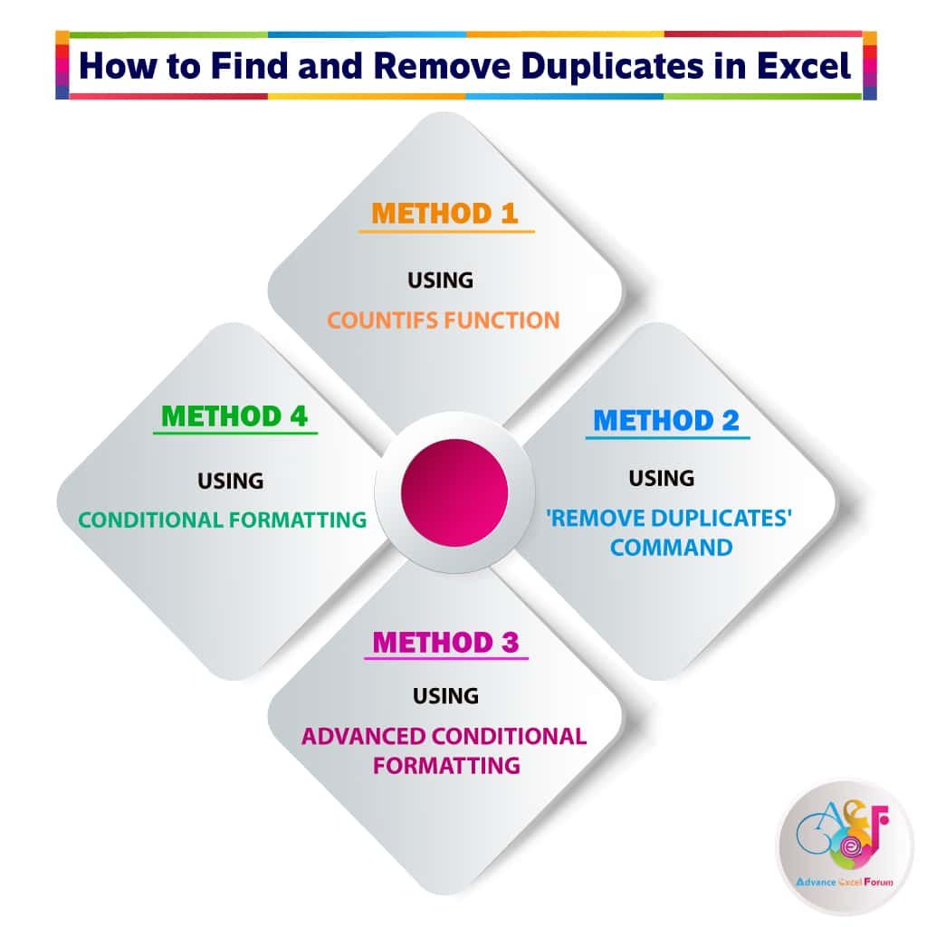
The question arises how to find and remove duplicates in Excel? When simplifying a table/dataset that contains many entries, or when compiling data from multiple sources, we might find that a table/dataset contains multiple matching entries.

We can easily find and remove duplicate data from a table/dataset by using any of the following methods: 

(01) HOW TO FIND AND REMOVE DUPLICATES IN EXCEL ➢ USING COUNTIFS FUNCTION

While working with a huge dataset, it is impossible to find out duplicates and removes them one by one. The COUNTIFS function is the best solution because it fills up the below requirement: 

⇒ we can easily find and highlight duplicates in Excel dataset. 

⇒ We have got a chance to recheck the duplicate data.

⇒ We can easily remove duplicates in Excel dataset without disturbing unique data.

■ Note: Instead of the COUNTIFS function, we can also apply the COUNTIF function. 

STEP 1: HOW TO FIND DUPLICATES IN EXCEL

Place an equality sign (=) in cell F2 and type ‘count…’, select COUNTIFS from the below suggestion list by the Down Arrow key (⬇) and then press the ‘Tab’ key.

■ Note: the upper or lower case does not matter in syntax, Excel by default considers it in upper case.

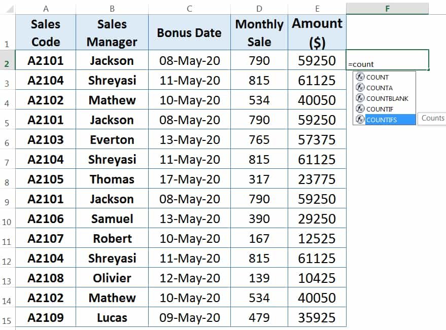
As a result, the COUNTIFS syntax appears with an open parenthesis.

Select the cell A2 as criteria_range1, the first argument of the COUNTIFS function. Then press full stop (.) from the keyboard, so Excel converts the cell reference into a range and the range starts from the same cell (or the same point) and it seems to be A2:A2.

Place a comma (,) to move to the next argument.

Again select cell A2 as criteria1, the second argument of COUNTIFS function.

■ Using Cell References

Simply select the starting cell reference of the criteria_range1 and press the F4 Key once which will convert the cell reference from the relative cell reference to the absolute cell reference.

Now the criteria_range1 seems to be $A$2:A2.

■ Note: We had detail discussed on Cell Reference in a separate tutorial, suggested you read this tutorial: 03 Types of Excel Cell Reference: Relative, Absolute & Mixed

Finally, press Enter to apply the formula in cell F2 and get the count value 1 as a result. 

■ Extend the Formula Downward till the End of the Range:

It is the best practice to extend the formula from a cell to the end of the range with the ‘Formulas and number formats’ in the Paste Special dialog box. 

Copy (Excel shortcut Ctrl+C) the cell F2 with formula ➪ Then makes a selection downward till to the end of the range with Shift+ Down arrow (⬇) ➪ After that either press Alt+E+S+R (sequentially press Alt, E, S, R) or  press Alt+Ctrl+V+R (Alt+Ctrl+V, then press R) which will select the ‘Formulas and number formats‘ option in the ‘Paste Special’ dialog box ➪ Click OK or press Enter to accept the formula. As a result, formula copied to the selected range without copying the cell formatting.

■ Note: We had detail discussed on Alt Key Excel Shortcuts in a separate tutorial, suggested you read this tutorial: 80+ Excel Shortcuts with ALT Key || Best Hotkey of Keyboard Shortcuts

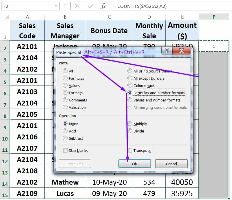
Alternatively, Copy (Ctrl+C) the cell F2 ➪ Then makes a selection downward till to the end of the range with Shift+ Down arrow (⬇) ➪ After that paste (Ctrl+V or simply press ‘Enter’). As a result, formula copied to the selected range with copying the same cell formatting. 

Alternatively, select the cell that has the formula we want to fill down to the range ➪ either double click on the fill handle or drag the fill handle down to the range. As a result, formula copied to the selected range with copying the same cell formatting. 

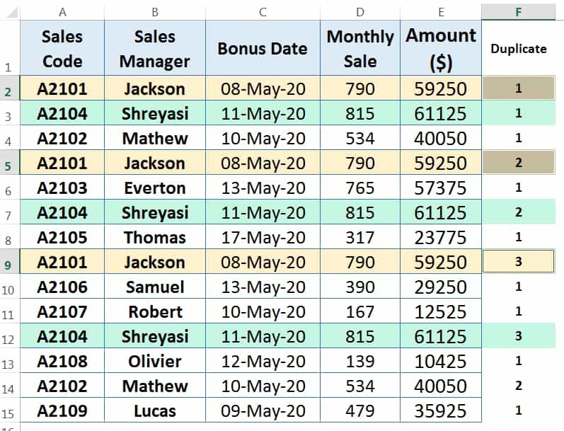
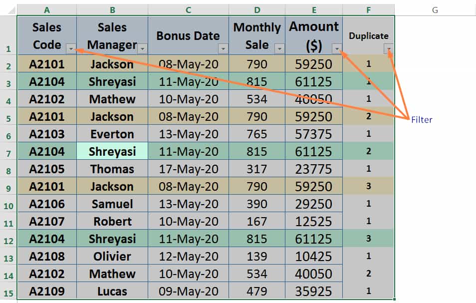
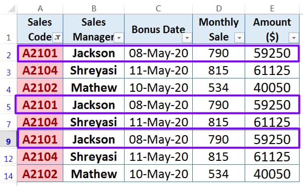
After copying the formula, we carefully notice that same duplicates in the dataset are marked in ascending order. For example, If we consider the Sales Manager Jackson, whose name  is duplicated three times in the dataset and the duplicate count is placed in ascending order likes 1, 2 and 3. So we should always keep the 1 value as a unique value and remove more than 1 value likes 2, 3, 4 etc. from the dataset as duplicates. 

STEP 2: HOW TO REMOVE DUPLICATES IN EXCEL

In the second step, we remove duplicates in Excel dataset with Excel Filter. 

It is the best practice to select the entire dataset with Ctrl+A ➪ Then press Ctrl+Shift+L (hold down the Ctrl and Shift keys and then press the L key) which will apply the Filter in the subject heading.

■ Note: We had detail discussed on Ctrl Key Excel Shortcuts in a separate tutorial, suggested you read this tutorial: 90+ Best Excel CTRL Shortcuts | Useful Keyboard Shortcuts |

Additionally, suggest you to read the usage of Excel Filter: 04 Simple to Advanced Methods: How to Filter in Excel?

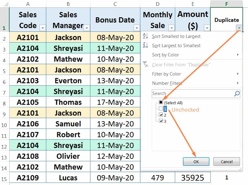
After applying the filter, open the filter list in column F by using the Alt+ Down arrow (⬇) or clicking on the filter drop-down arrow ➪ Then unselect the value 1 (considers as a unique value) ➪ Finally, press OK.  

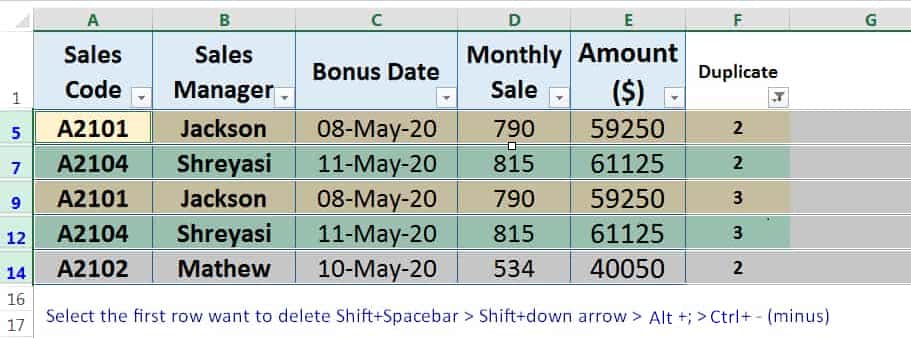
As a result, all the duplicates are filtered ➪ Select the first row which one wants to delete either with the Shift+Spacebar or clicking on the row number ➪ Then select other rows downward with the Ctrl+Shift+Down arrow (⬇) or Shift+Down arrow (⬇) or Shift+Page Down ➪ After selection, press Alt+; (semicolon) for select visible cells only ➪ Finally, press Ctrl+- (minus) which will delete the all the rows with duplicates.

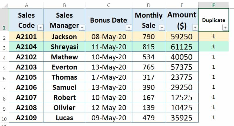
After deleting the rows, clear the filter with the Excel shortcut Alt+A+C (sequentially press Alt, A, C) or press Alt+D+F+S (sequentially press Alt, D, F, S).

As a result, only the unique values are present in the dataset.  

(02) HOW TO FIND AND REMOVE DUPLICATES IN EXCEL ➢ USING ‘REMOVE DUPLICATES’ COMMAND

We can remove duplicates in Excel dataset with the ‘Remove Duplicates‘ command in the Data Tools group under the Data tab.

(i) Click any cell in the dataset we want to work with.

(ii) Go to the Data tab ➪ Click Remove Duplicates in the Data Tools group ➪ The Remove Duplicates dialog box appears. In the Remove Duplicates dialog box, verify that My data has headers is selected and The Excel by default selected all columns.

Note: We can customize our column selection. First, click Unselect All and then check or uncheck the columns we want Excel to examine.

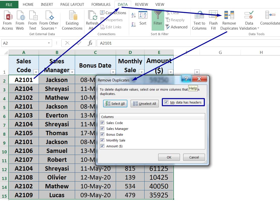
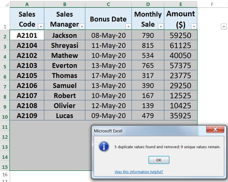
(iii) Click OK. Excel looks for and removes duplicates.

A message appears reporting how many duplicate records were removed (if any) and how many unique values remain.

(03) HOW TO FIND AND REMOVE DUPLICATES IN EXCEL ➢ USING ADVANCED CONDITIONAL FORMATTING

Another method to find and remove duplicates in Excel is Conditional Formatting.

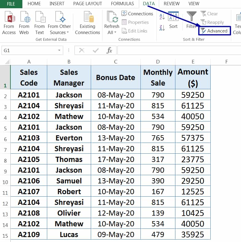
(i) Go to the Data tab ➪ Click Advanced in the Sort & Filter group which will open the Advanced Filter dialog box.

(ii) First, select the Copy to another location radio button.

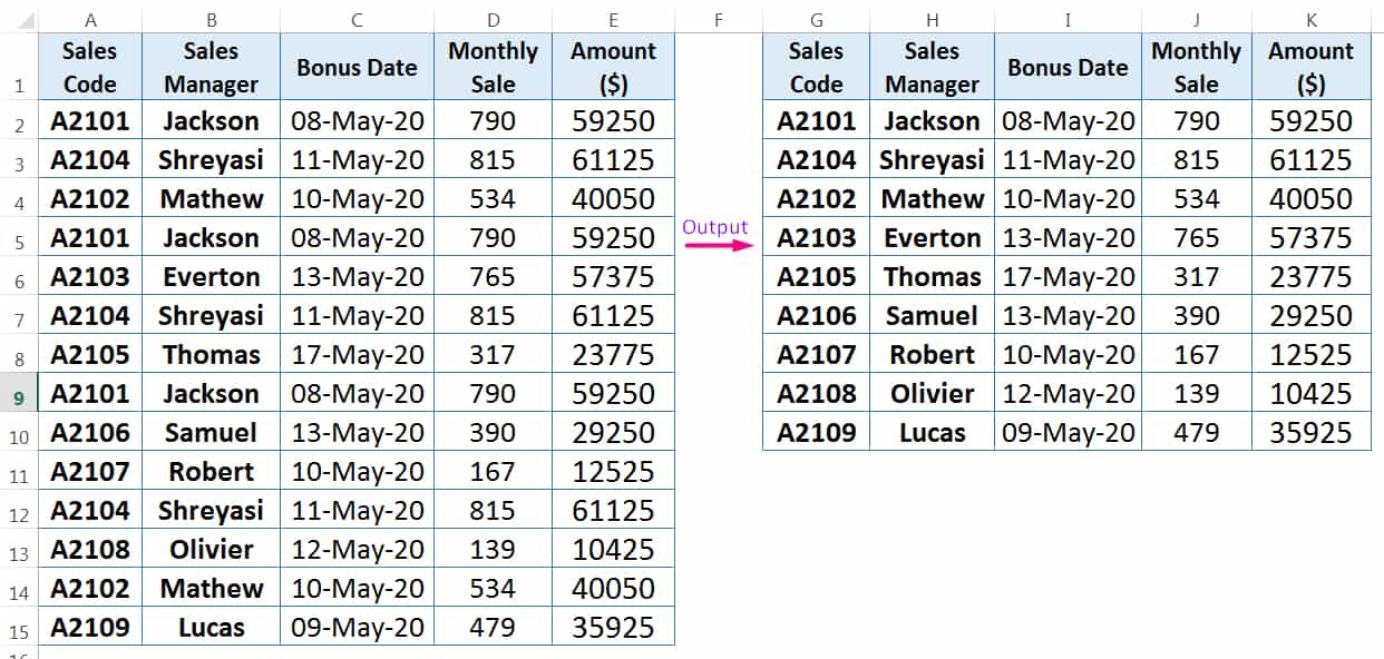
Then click in the List range box and select the dataset range (in this case we select the range A1:E15).

Then click in the Copy to box and select a cell of the new location (in this case we select the cell G1).

Select the Unique records only checkbox.

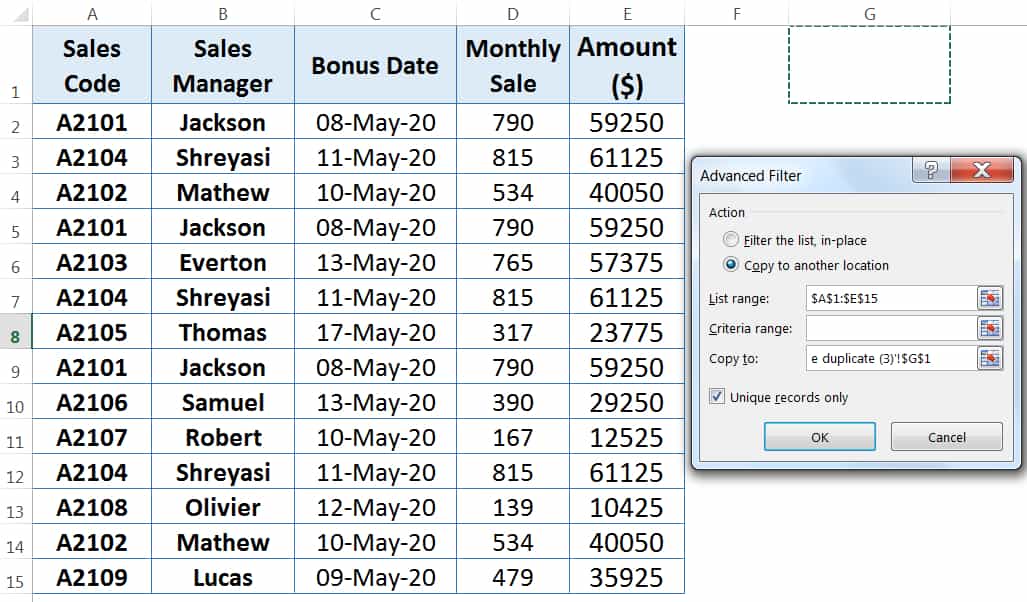
(iii) Finally, click OK or press Enter. 

As a result, Excel removes all the duplicates from the dataset to a new location. 

■ Note: We had detail discussed on Conditional Formatting in a separate tutorial, suggested you read this tutorial: 08 Best Examples: How to Use Excel Conditional Formatting?

(04) HOW TO FIND AND HIGHLIGHT DUPLICATES IN EXCEL ➢ USING CONDITIONAL FORMATTING

This method only helps us to find and highlight duplicates in Excel, but it fails to remove duplicates from the dataset. Actually, this method is useful for data entry purposes. If we put any duplicate entry, the cell formatting will be changed and instantly alarming us this entry is a duplicate.

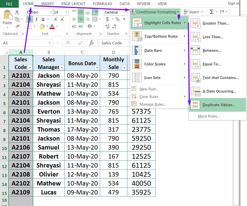
Either select only the range or select the entire column A with the shortcut Ctrl+Spacebar or clicking on the column header A ➪ Go to the Home tab ➪ Click Conditional Formatting drop-down ➪ Point over Highlight Cells Rules and a list opens ➪ Select Duplicate Values.

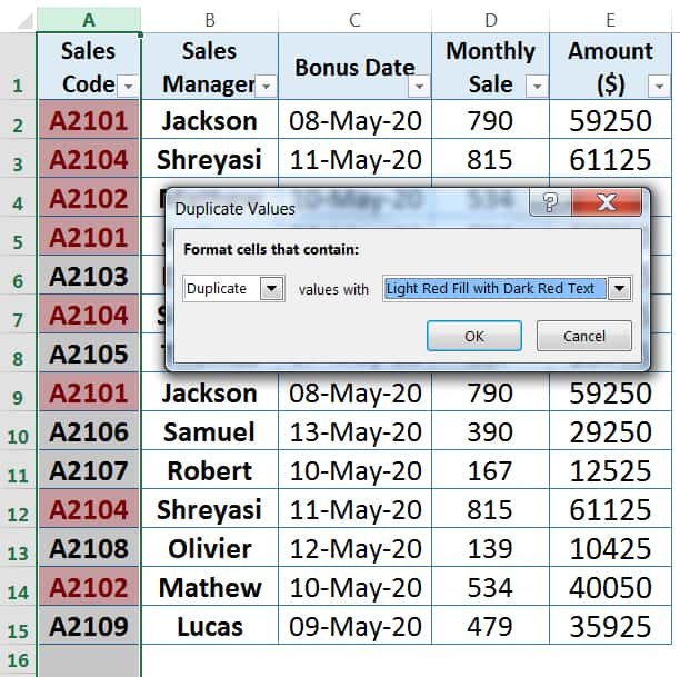
As a result, a Duplicate Values dialog box opens ➪ Consider all the default setting (or choose the different cell formatting using the values with drop-down) ➪ Click OK which will mark all the duplicates with a specific color.

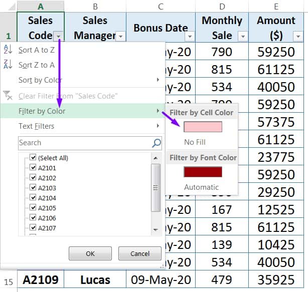
Apply the filter using Excel shortcut Alt+D+L (sequentially press Alt, D, L) and open the filter drop-down list by pressing Alt+ ⬇ or clicking on it ➪ Point over Filter by Color ➪ Choose color from the Filter by Cell Color. As a result, all the duplicate values filtered out. 

If we try to delete all the duplicates by color, then the unique item and its duplicates are removed, which means the actual entry is deleted from the dataset. In the given example, there are three entries of Sales Manager Jackson, we consider one is unique and the rest two are duplicates. If we delete by color, three entries of Jackson have been removed which means Jackson entry have been totally removed from the dataset.