TABLE OF CONTENTS:
Toggle(I). WHAT IS EXCEL CONDITIONAL FORMATTING?
In Excel, “formatting” means visually changing a cell. Some examples of format are:
➢ Alignment of the text (left, right, middle or justified)
➢ Fill the cell with one color (Fill Color)
➢ Modify the font color (Font Color)
➢ Bold, Italic and Underline the text
➢ Modify the size of the text (Font Size)
➢ Modify the font of the text (Font)
➢ Apply borders to the cell
➢ Wrapping the text
The Excel conditional formatting is formatting that changes selectively and automatically depending on the contents of the cells, which means the Excel Conditional formatting automatically format a cell when the applied condition(s) are met.
We can apply a single condition or multiple conditions. We can use the preset conditions (or rules) provided by Excel or customize them through the “Conditional Formatting Rules Manager” dialog box where we set the order of multiple rules.
The term is called conditional because the formatting only displays when a condition is met. This is similar logic to the IF function. If the logical or conditional test is true, the function produces one result. If the logical or conditional test is false, the function produces another result. With conditional formatting, if the condition is true, Excel formats the cell automatically based on that condition. If the condition is false, Excel does not format the cell. If you change a value in a conditionally formatted cell, Excel examines the new value to see if it should apply the conditional format.
Conditionals in Excel are logical sequences that normally follow the pattern “If the CONDITION is met, then Excel FORMATS the cell”. There are a few types of conditions:
➢ The value of the cell is lower or higher than another;
➢ The value of one cell is the same as another;
➢ The cell contains a certain letter, word, or phrase;
➢ The values are duplicated within a group of several cells;
➢ The values are within a range of dates;
➢ The values are the minimum or maximum values within a group of cells;
➢ Many other conditions can be added.
(II). MERITS OF EXCEL CONDITIONAL FORMATTING
• With the conditional formatting tool it is extremely easy to automatically highlight the information that we want.
• Conditional formatting offers a quick and visually comfortable solution to analyze and present information.
Tips:
• Although conditional formatting helps identify trends, we should use this feature wisely and sparingly.
• Apply conditional formatting only when we want to emphasize important data. When we decide to apply conditional formatting, think about which category is best to highlight the data.
(III). HOW TO ACTIVATE THE EXCEL CONDITIONAL FORMATTING TOOL?
(01). The first step is to select a group of cells or a single cell that contains the value(s) and we want to format.
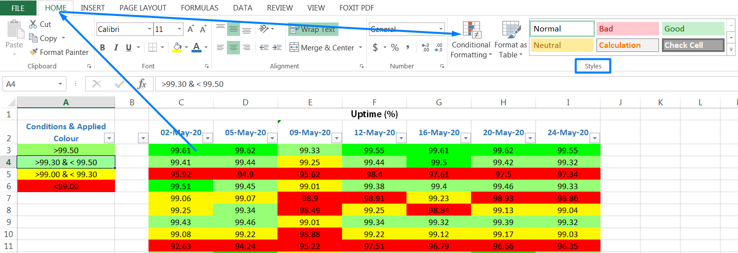
(02). The second step is to find the tool within the Excel menu. To find conditional formatting within Excel follows this path:
➢ Method 1:
Select cell(s) ➪ Home ➪ Styles ➪ Conditional Formatting drop-down list to specify a rule.
➢ Method 2:
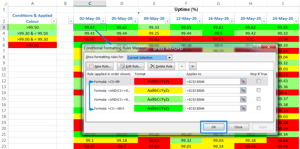
Select cell(s) ➪ press sequentially Alt+O+D (sequentially press Alt, O, D) which will open ‘Conditional Formatting Rules Manager’.
(03) After clicking on the “Conditional Formatting” drop-down, the following menu will be displayed and we can choose any of the options.
The menu has 3 sections that include 8 options in total.

1ST SECTION
The first section includes the following 2 options:
➢ Highlight Cell Rules:
This option has the most flexible conditional formatting tools. We can highlight the cell(s) with a fill color, font color, or border (such as Light red Fill with Dark red text) based on its value.
For example, if a cell is less than, equal to or greater than a certain number (value); between two values; or contains duplicate values; or text that contains particular characters; or dates when a date meets a particular condition, such as in the last week, last month, next week, etc.
➢ Top/Bottom Rules:
It allows us to identify a certain amount of the upper and lower elements. For example, formats cells with values in the top 10 items, top 10%, bottom 10 items, bottom 10%, above average, or below average.
Note: We can change the exact values to format the top or bottom items or percentages, such as the top 5 or bottom 15%.
2ND SECTION
This section includes 3 options:
➢ Data Bars:
Applies graphic bar (gradient or solid fill bar) directly in the cells, proportional to the cell’s value.
According to the value, the bar becomes larger or smaller.
➢ Color Scales:
Applies background color, proportional to the cell’s value.
We have the option to use scales of 2 or 3 colors.
Formats different cells with different colors, assigning one color to the lowest group of values and another color to the highest group of values, with gradient colors to other values.
➢ Icon Sets:
Displays icons directly in the cells. The icons depend on the cell’s value.
There is a large variety of icons that we can use to identify the higher, the lower, and the average values.
3RD SECTION
When we order Excel to apply a conditional formatting option (from the 1st or 2nd section) to a group of cells, Excel by default creating a new CONDITIONAL FORMATTING RULE.
The 3rd section focuses on 3 options:
➢ New Rule:
This option allows to create own conditional formatting rules (including rules based on a logical formula) and modify some parameters.
➢ Clear Rules:
It is the option that allows us to choose which rules to delete, that is, in which cells no longer want to use conditional formatting.
➢ Manage Rules:
Displays the Conditional Formatting Rules Manager dialog box, in which you create new conditional formatting rules, edit rules, or delete rules.
(IV). EXCEL CONDITIONAL FORMATTING BASED ON ANOTHER CELL RANGE
A. HIGHLIGHT CELLS RULES
The Highlight Cells Rules option enables us to apply a highlight to cells that meet a condition, such as cells containing values greater than a particular value. This option contains predefined combinations of fill colors, font colors, and/or borders.
The Highlight Cell Rules option has 7 quick preset rules that we can quickly access.

• GREATER THAN
This rule allows Excel to automatically highlight (with the selected color) all the cells that are greater than a value or a cell.
For example, a table with values (percentage %) from 0 to 100 is presented, and we need to highlight the values above 99.5 (%). In that case, we should do the following:
Step 1: Select the group of cells or a cell.
Step 2: Home ➪ Styles ➪ Conditional Formatting ➪ Highlight Cells Rules ➪ Greater Than…
Step 3: Write the value 99.5.

• LESS THAN
This rule allows Excel to automatically highlight all cells that are lower than a specific value or a cell.
For example, a table with values (percentage %) from 0 to 100 is presented, and we need to highlight the values above 99 (%). In that case, we should do the following:
Step 1: Select the group of cells or a single cell.
Step 2: Home ➪ Styles ➪ Conditional Formatting ➪ Highlight Cells Rules ➪ Less Than…
Step 3: Write the value 99.

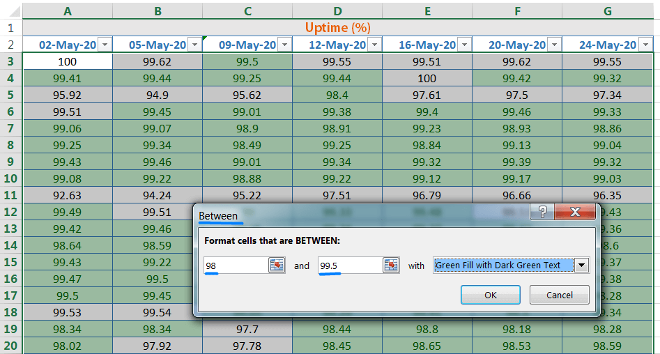
• BETWEEN
This rule allows Excel to automatically highlight all the cells that are between two values or two cells that we choose.
For example, a table with values (percentage %) from 0 to 100 is presented, and we need to highlight the values between 98 and 99.5 (%). In that case, we should enhance the following:
Step 1: Select the group of cells or a single cell.
Step 2: Home ➪ Styles ➪ Conditional Formatting ➪ Highlight Cells Rules ➪ Between…
Step 3: Write the value 98 and 99.5.
• EQUAL TO
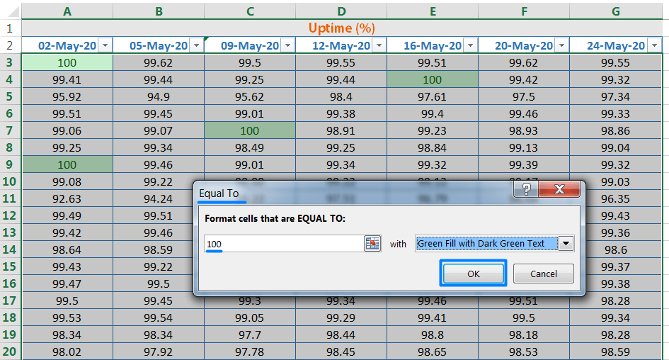
This rule allows Excel to automatically highlight the cells that are equal to a value or another cell that we indicate.
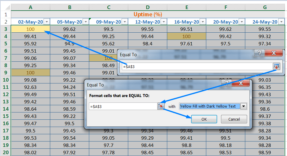
In the example, we need to highlight the values that are equal to the value 100. We can do it in 2 ways:
➢ Method 1: Manually type the Value
Step 1: Select the group of cells or a single cell.
Step 2: Home ➪ Conditional Formatting ➪ Highlight Cells Rules ➪ Equal To…
Step 3: Write the value 100.
➢ Method 2: Using the Cell Reference
Step 1: Select the group of cells or a single cell.
Step 2: Home ➪ Styles ➪ Conditional Formatting ➪ Highlight Cells Rules ➪ Equal To…
Step 3: Select the cell A3 as a cell reference, where A3 refers to the value 100.
• TEXT THAT CONTAINS NUMBER / TEXT
This rule allows Excel to automatically highlight the cells that contain the text or number we want. We can even be as specific as choosing the text to be found only in the middle or at the end.
➢ EXCEL CONDITIONAL FORMATTING BASED ON NUMBER
Step 1: Select the group of cells or a single cell.
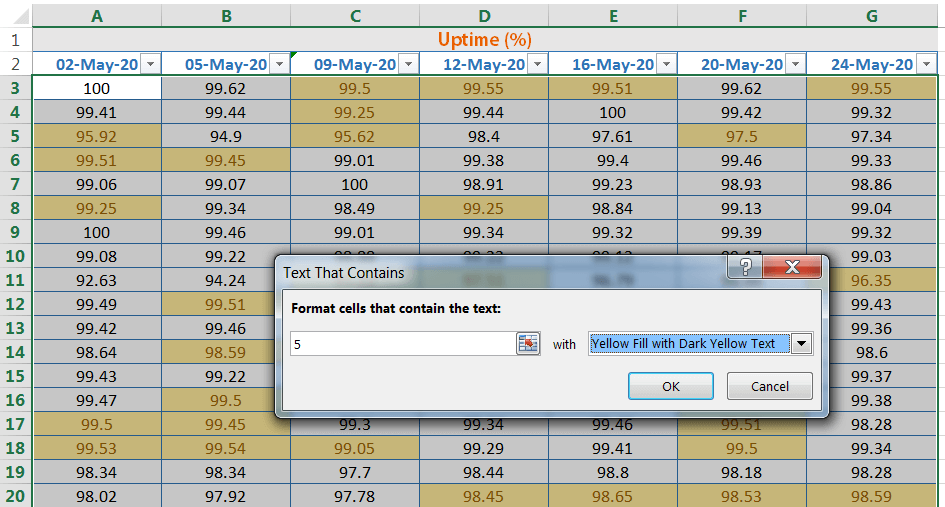
Step 2: Home ➪ Styles ➪ Conditional Formatting ➪ Highlight Cells Rules ➪ Text that Contains…
Step 3: Write the text or number. Here we wrote the number ‘5‘ in this example, thus the 99.5, 99.51, 99.55, 95.92, 99.25, etc., values were highlighted because they include the number 5.
➢ EXCEL CONDITIONAL FORMATTING BASED ON TEXT
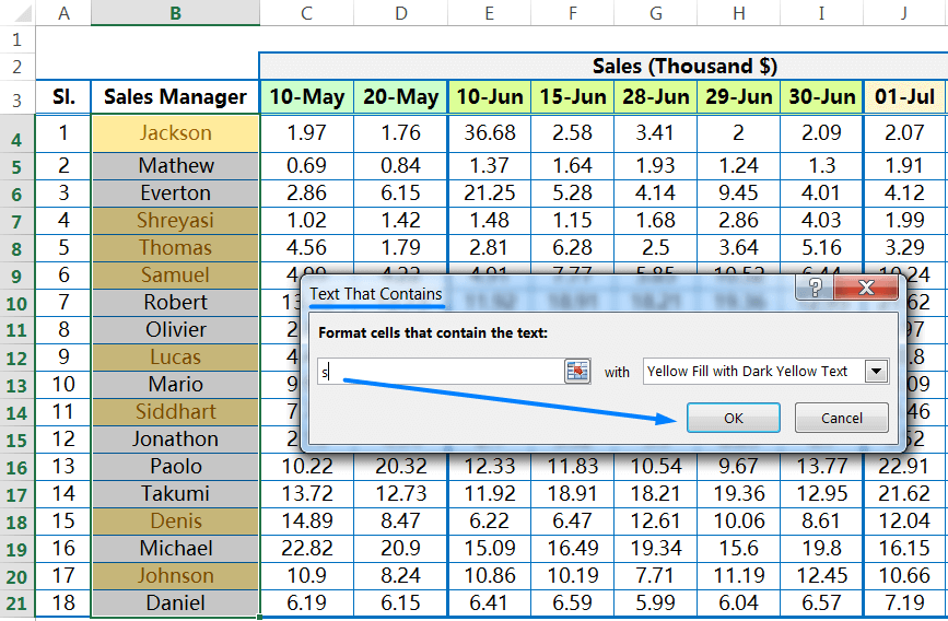
Similarly, we type the text ‘s’ for this example, thus all the names were highlighted with text ‘s’. For example, Jackson, Shreyasi, Thomas, Samuel, Lucas, etc.
• A DATE OCCURRING
➢ EXCEL CONDITIONAL FORMATTING BASED ON DATE
This rule allows Excel to automatically highlight the cells that are within a certain range of dates that we selected.
There are the following 10 options: Yesterday, Today, Tomorrow, In the last 7 days, Last week, This week, Next week, Last month, This Month, Next month.
Step 1: Select the group of cells or a single cell.
Step 2: Home ➪ Styles ➪ Conditional Formatting ➪ Highlight Cells Rules ➪ A date occurring…
Step 3: Select any of the options. However, we selected Last week in this example.

• DUPLICATE VALUES
This rule allows Excel to automatically highlight the cells that are repeated (more than once) within a group. It can be text, date and value. Also, by contrast, we can fill in the cells that are NOT repeated, that is, the unique values.
Step 1: Select the group of cells or a single cell.
Step 2: Home ➪ Styles ➪ Conditional Formatting ➪ Highlight Cells Rules ➪ Duplicate Values…
➢ Example 1: Considering the Date (highlight the duplicate date)

➢ Example 2: Considering the Text (highlight the duplicate text)

• MORE RULES
Click on the option ‘More Rules’ which will open the ‘New Formatting Rule’ dialog box that allows us to use conditional formatting with other variants such as:
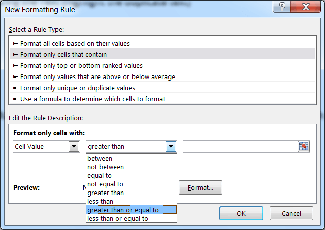
➢ Greater than or equal to
➢ Less than or equal to
➢ Empty cells
➢ Non Empty cells
➢ Cells with errors
➢ Cells without errors
B. TOP/BOTTOM RULES
A top/bottom rule is one that applies a format to cells that rank in the top or bottom values in a range.
For example, the Top/Bottom Rules option enables us to specify the top or bottom number, top or bottom percentage, or values that are above or below the average value in a specified range.
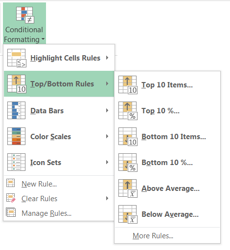
The Top / Bottom Rules option includes 6 quick access rules.
• TOP 10 ITEMS
The “Top 10 Items” option is used to automatically highlight the cells with the 10 highest in a range.
However, the default value is 10, but we can change the value as per requirement.
• TOP 10%
It works almost like the “Top 10 Items”. In this case, you can apply a conditional format to 10% of the highest values.
However, the default value is 10, but we can change the value as per requirement.
• BOTTOM 10 ITEMS
It works in exactly the same way as “Top 10 Items”, with the difference that this rule highlights the 10 lowest values in a range.
However, the default value is 10, but we can change the value as per requirement.
• BOTTOM 10%
It works in exactly the same way as “Top 10%”, with the difference that this rule highlights 10% of the lower values or the percentage of values in a range.
However, the default value is 10, but we can change the value as per requirement.
• ABOVE AVERAGE
This rule is very useful because it performs 2 functions at the same time. First, calculate the average of the group of selected cells, and second apply conditional formatting to the cells that are above that average.
Any modification of the values in the group of cells will automatically modify the average.
• BELOW AVERAGE
This rule first calculates the average of the values of the group of selected cells and then applies conditional formatting to the values that are below the average.
Any modification of the values in the group of cells will automatically modify the average.
C. DATA BARS
The second section of the Conditional Formatting menu has 3 options: Data Bars, Color Scales, and Icon Sets.
Any of these 3 options need to be used with a group of cells, it cannot be used with individual cells. The reason for this is because the conditional formatting that is applied to each cell will depend on its size (value) in relation to the others in the group.
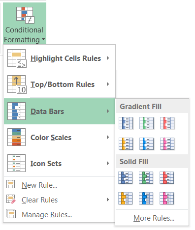
The Data Bars option creates a mini horizontal bar within each cell of the group as if a small mini graphic was formed. The length of the bar is based on the value of the cell, relative to the other values in the range.
Excel locates the largest value and displays the widest data bar in that cell. Excel, then finding the smallest value and displays the smallest data bar in that cell.
If we change the values, Excel updates the data bar widths. Excel uses the same color for each data bar, but each bar differs in size based on the value in the respective cells.
The type of bar can be a solid fill or gradient fill. Negative values can also be included, so the bar will grow to the left.
Step 1: Select the group of cells.
Step 2: Home ➪ Styles ➪ Conditional Formatting ➪ Highlight Cells Rules ➪ Data Bars
Step 3: Showing 2 options: Gradient Fill and Solid Fill. Select any of the options.
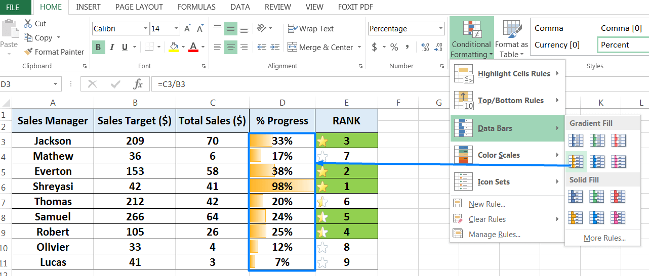
One last important fact is that we can configure the size of the bars. In this case, we should change the minimum type from ‘Automatic’ (which is established by default) to ‘Lowest value’. As a result, the minimum of the bars equal to 0, in other words, for a cell to appear without the bar, its value must be zero.
In the given example, we modified the minimum value. As a result, the lowest value 7% (the minimum value of the group), which appears without any bar, but the rest of the values showing bars by default.
➢ HOW TO CHANGE THE MINIMUM VALUE?
Step 1: Select the group of cells and choose any of the Data Bars, the minimum value will automatically be 0.
Step 2: Then, either we press sequentially Alt+O+D (Alt, O, D) which will open ‘Conditional Formatting Rules Manager‘ dialog box;
Or, Home ➪ Styles ➪ Conditional Formatting ➪ Manage Rules ➪ Conditional Formatting Rules Manager.

Step 3: After opening the ‘Conditional Formatting Rules Manager’ dialog box, either double click on the rule that has been created; or click on ‘Edit Rule…’, which will open the ‘Edit Formatting Rule‘ dialog box

Step 4: In the parameter Minimum Value set by default “Automatic” but we must change it to “Lowest Value“. Click on ‘OK’ and then on ‘Apply’.
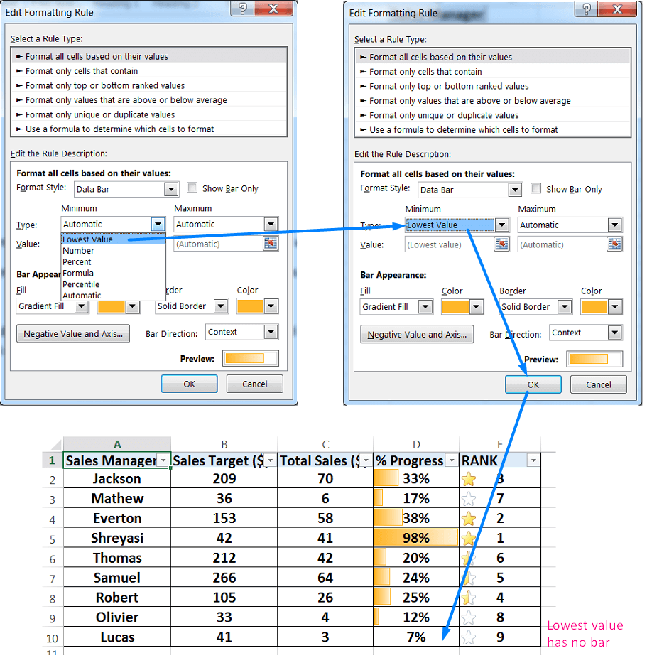
As a result, the lowest value (e.g., 7%) appears without any bar. If we observed the two images with the same values, but the second configuration allows us to see the differences easily.
Any of the 2 forms fulfill the objective of displaying the information visually, it only depends on what we prefer.
For additional choices, click the More Rules option, which displays the New Formatting Rule dialog box. Use this dialog box to
i) Show the bar only (hide the numbers)
ii) Specify Minimum and Maximum values for the scaling
Notice that there’s a Type list for both the Minimum and Maximum. The type determines how Excel applies the data bars. Excel provides the following six options:
➢ Automatic—This is the default choice, and it means that Excel chooses the type automatically based on the data.
➢ Lowest/Highest Value—With this bar type, the lowest value in the range gets the shortest data bar, and the highest value in the range gets the longest data bar. This is the most common type, and it’s the type Excel usually selects when the ‘Type’ list values set to Automatic.
➢ Number—Use this type to base the data bar lengths on values that we specify in the two Value text boxes.
For the Shortest Bar, any cell in the range that has a value less than or equal to the value we specify and will get the shortest data bar. Similarly, for the Longest Bar, any cell in the range that has a value greater than or equal to the value we specify and will get the longest data bar.
➢ Percent—Use this type to base the data bar lengths on a percentage of the largest value in the range.
For the Shortest Bar, any cell in the range that has a relative value less than or equal to the specified percentage we specify will get the shortest data bar. For example, if we specify 15 percent and the largest value in the range is 1,000 so any cell with a value of 150 or less will get the shortest data bar.
For the Longest Bar, any cell in the range that has a relative value greater than or equal to the percentage we specify will get the longest data bar. For example, if we specify 80 percent and the largest value in the range is 1,000, so any cell with a value of 800 or more will get the longest data bar.
➢ Formula—Use this type to base the data bar lengths on a formula.
➢ Percentile—Use this type to base the data bar lengths on the percentile within which each cell value falls given the overall range of the values. In this case, Excel ranks all the values in the range and assigns each cell a position within the ranking.

For the Shortest Bar, any cell in the range that has a rank less than or equal to the percentile we specify will get the shortest data bar. For example, if data have 100 values, and specify the 20th percentile, the cells ranked 20th or less will get the shortest data bar.
For the Longest Bar, any cell in the range that has a rank greater than or equal to the percentile we specify will get the longest data bar. For example, if data have 100 values and specify the 80th percentile, any cell ranked 80th or higher will get the longest data bar.

iii) Change the appearance of the bars
iv) Specify how negative values on the axis are handled
v) Specify the direction of the bars
If we make adjustments in this dialog box, we can use the Preview button to see the formats before commit to them by clicking OK.
➢ CONCLUSION:
• Data Bars create a horizontal bar within the cell, in the form of a mini graphic.
• The higher the value, the more the bar grows to the right.
• Negative values can be included.
• The empty bars can be the values 0 or the minimum values of the group, depending on the selected configuration.
D. COLOR SCALES
➢ EXCEL CONDITIONAL FORMATTING COLOR SCALE BASED ON ANOTHER CELL
Color scales are another form of Conditional Format for a group of cells. Color scales format cells with different colors based on the relative value of a cell compared to other selected cells.
They are used to identify the highest, lowest, and average values.
We can apply a two- or three-color scale. This scale assists in comparing a range of cells using gradations of those colors. The shade of the color represents higher or lower values.
In the given figure, for example, the red color scale displays for the lowest values, the green color displays for the highest values, and gradients of yellow and orange represent the middle range of values. Use color scales to understand variation in the data to identify trends, for example, to view good progress and weak progress as well.

➢ HOW TO MODIFY THE COLOR SCALES?
Select the group of cells and choose any of the Color Scales.
Like the Data Bars, the minimum and maximum values of the Color Scales can be configured with the option “Manage Rules”. In this case, either we press sequentially Alt+O+D (Alt, O, D) which will open the ‘Conditional Formatting Rules Manager‘ dialog box; or Home ➪ Styles ➪ Conditional Formatting ➪ Manage Rules ➪ Conditional Formatting Rules Manager.
After opening the ‘Conditional Formatting Rules Manager’ dialog box, either double click on the rule that has been created; or click on ‘Edit Rule…’, which will open the ‘Edit Formatting Rule‘ dialog box.
We can set a 2-Color Scale or 3-Color Scale from the ‘Format Style’ drop-down menu.
By default, the minimum and the maximum of the color scales are set to be the lowest value and the highest value of the group of cells.
We can change the color as per our choice. Click on ‘OK’ and then on ‘Apply’.
Please note that if we select a scale of 2 colors (orange and white), no matter how high the values are, the lowest value will be filled with white, because by default Excel considers it as the “minimum” for the color scale.

➢ CONCLUSION:
• Color scales fill the cell with gradient color, depending on the cell value.
• There are scales of 2 and 3 colors.
• The minimum and maximum of the color scale can be configured.
E. ICON SETS
Icon sets are symbols or signs that classify data into three, four, or five categories, based on the values in a range. Excel determines the categories of value ranges and assigns an icon to each range.
There are 4 alternative options:
• Directional icons
• Shape icons (which are actually color changes)
• Indicators
• Ratings
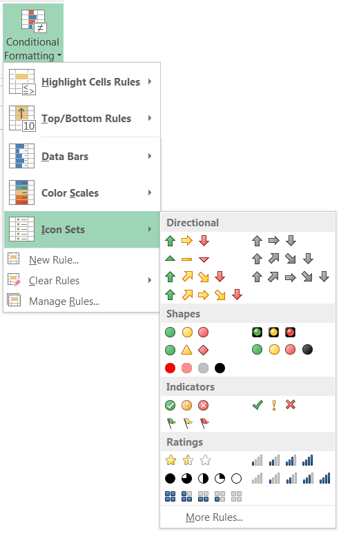
In general, we can use a group of icons based on the requirement.
The most important thing we should understand about the Excel conditional formatting with icons is that they can be used in two main ways:
• Group: Relating values in a group (like color scales).
• As an indicator: Establishing parameters (minimum and maximum) in advance to define what performs well and what performs badly.
In the given example, the 3-star icon- set was applied to the RANK column. Excel by default arranges the stars from lowest to highest values. As we show the ranking of performance, the lowest value is the highest performer, which means rank 1 is the best performer and rank 9 is the poor performer. So in this case, we arrange the icons in the reverse order.
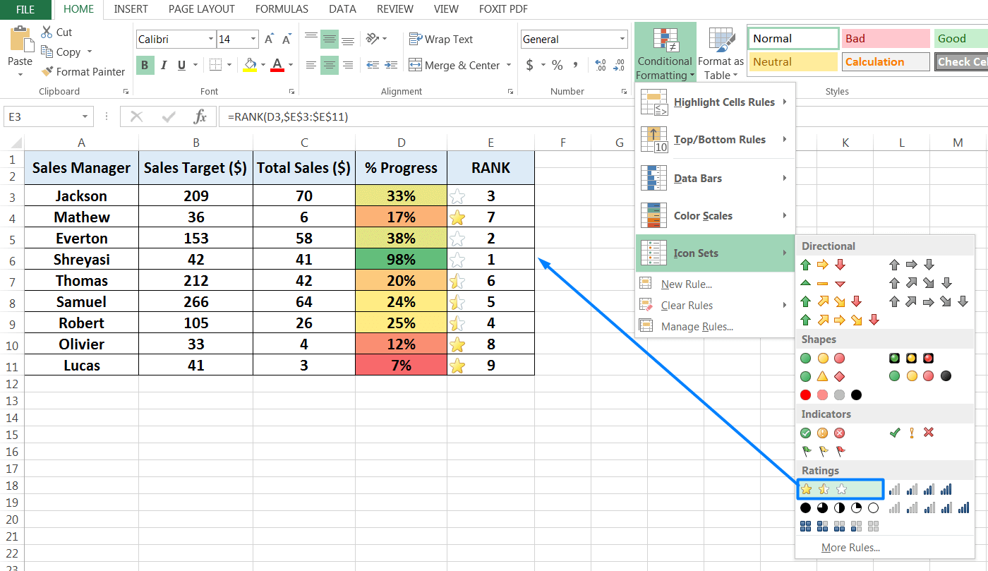
Step 1: Select the group of cells and choose the 3-star icon from the ‘Ratings’ option.
Step 2: Then either we press sequentially Alt+O+D (Alt, O, D) which will open ‘Conditional Formatting Rules Manager‘ dialog box;
Or Home ➪ Styles ➪ Conditional Formatting ➪ Manage Rules ➪ Conditional Formatting Rules Manager.
Step 3: After opening the ‘Conditional Formatting Rules Manager’ dialog box, either double click on the rule that has been created; or click on ‘Edit Rule…’, which will open the ‘Edit Formatting Rule‘ dialog box.
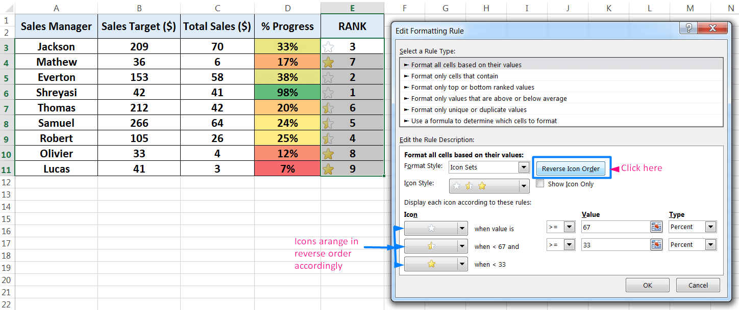
Step 4: Click on ‘Reverse Icon Order’ as a result, icons are arranged in reverse order. Click on ‘OK’ and then on ‘Apply’ to get the effect.

➢ CONCLUSION:
• Icon Sets work similarly to the Color Scales, but the icons are easier to recognize visually.
• We can use them in groups.
• We can use them as an indicator
• We can reverse the icon order as per requirement.
F. NEW RULE
The default conditional formatting categories provide a variety of options. Excel also enables us to create our own rules to specify different fill colors, borders, or another formatting if we do not want the default settings.
➢ HOW TO CREATE THE NEW RULE?
Excel provides 4 ways to create a New Rule.
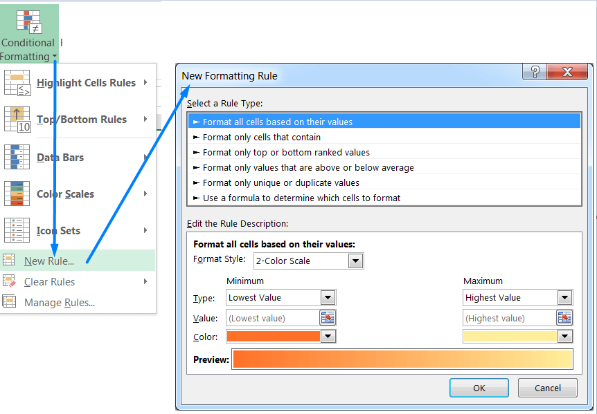
• Method 1: Home ➪ Styles ➪ Conditional Formatting ➪ New Rule… ➪ ‘New Formatting Rule‘ dialog box.
• Method 2: Home ➪ Styles ➪ Conditional Formatting ➪ Manage Rules ➪ ‘Conditional Formatting Rules Manager’ dialog box ➪ New Rule… ➪ ‘New Formatting Rule‘ dialog box.
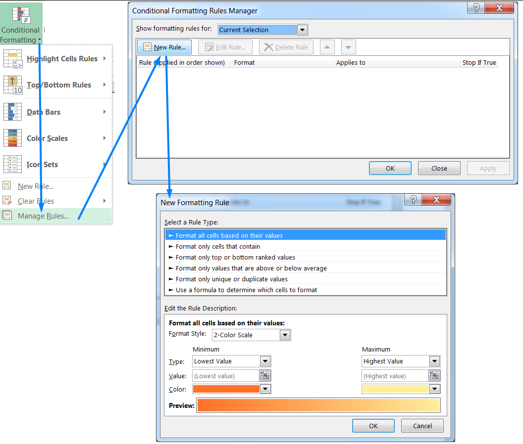
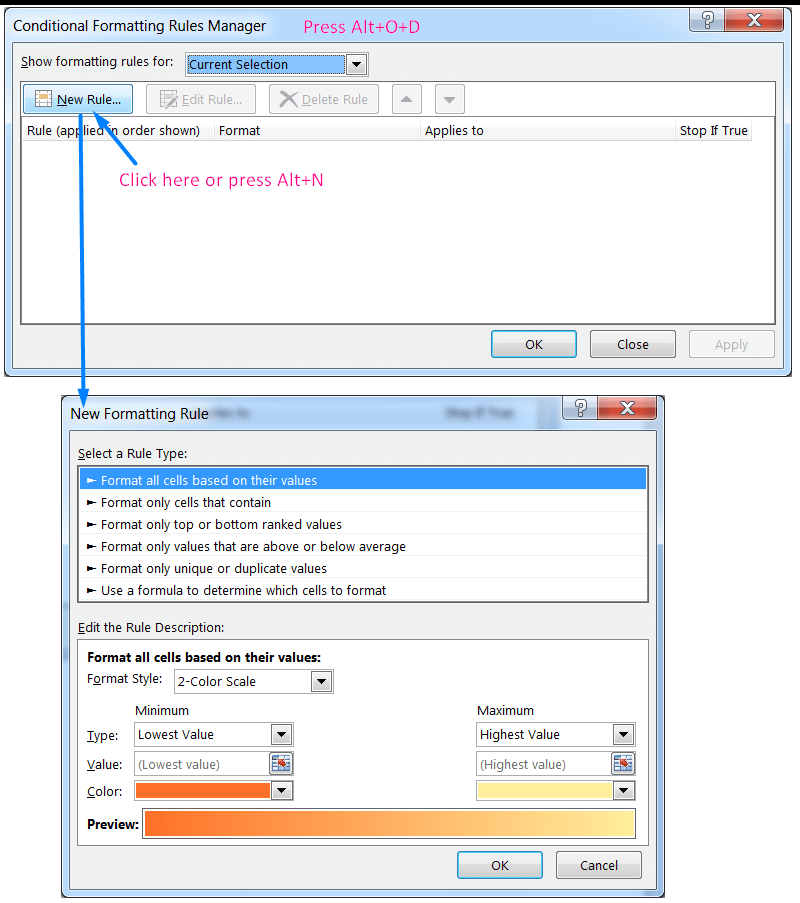
• Method 3: Using Excel shortcut Alt+O+D (sequentially press Alt, O, D) which will open the ‘Conditional Formatting Rules Manager’ dialog box ➪ then press Alt+N which will open ‘New Formatting Rule‘ dialog box.
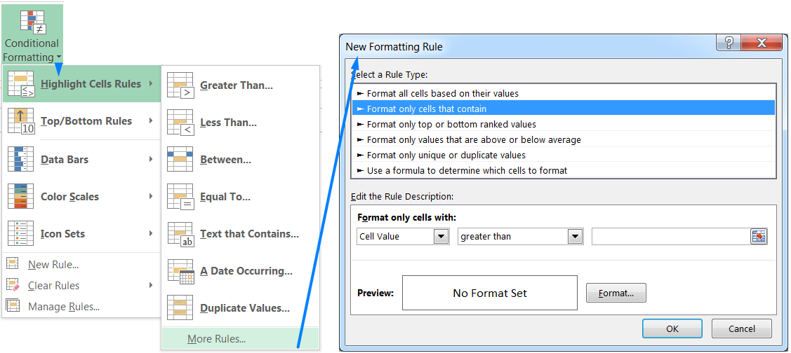
• Method 4: Click Conditional Formatting in the Styles group, select any rule category, such as Highlight Cells Rules, and then select More Rules (Home ➪ Styles ➪ Conditional Formatting ➪ Highlight Cells Rules ➪ More Rules…➪ ‘New Formatting Rule‘ dialog box).
When creating a new rule, the ‘New Formatting Rule’ dialog box opens so that we can define the conditional formatting rule.
First, select a rule type, such as Format all cells based on their values. The Edit the Rule Description section changes, based on the rule type we select. With the default rule type selected, but we can specify the format style (2-Color Scale, 3-Color Scale, Data Bar, or Icon Sets). Then specify the minimum and maximum values, the fill colors for color sets or data bars, or the icons for icon sets. After editing the rule description, click ‘OK’ to save the new conditional format.
If we select any rule type except the Format all cells based on their values rule, the dialog box contains a ‘Format‘ button. When we click ‘Format’, the Format Cells dialog box opens so that we can specify the number, font, border, and fill formats apply the rule.
➢ RULE TYPES IN THE NEW RULE:
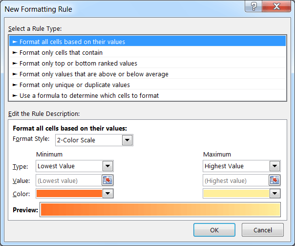
Here is a summary of the rule types:
➢ Format all cells based on their Values:
Use this rule type to create rules that display data bars, color scales, or icon sets.
➢ Format only cells that Contain:
Use this rule type to create rules that format cells based on mathematical comparisons (greater than, less than, greater than or equal to, less than or equal to, equal to, not equal to, between, not between). We can also create rules based on text, dates, blanks, non-blanks, and errors.
➢ Format only Top- or Bottom-ranked Values:
Use this rule type to create rules that involve identifying cells in the top n, top n%, bottom n, and bottom n%.
➢ Format only values that are Above or Below Average:
Use this rule type to create rules that identify cells that are above average, below average, or within a specified standard deviation from the average.
➢ Format only Unique or Duplicate Values:
Use this rule type to create rules that format unique or duplicate values in a range.
➢ Use a formula to determine which cells to format:
Use this rule type to create rules based on a logical formula.
G. MANAGE RULES (EDIT, DELETE & CREATE NEW RULES)
Periodically conditional formatting rules may need to be updated, moved, or completely deleted.
Moreover, we can manage the hierarchy of the rules, making some more important than others. In other words, we can order Excel what rules to apply in case two or more rules are activated in the same cell.
➢ USAGE OF MANAGE RULES:
• It helps to edit a conditional formatting rule
• It helps to change the order in which conditional formatting rules are applied
• It helps to delete a conditional formatting rule one by one.
➢ HOW TO CREATE MANAGE RULES?
• Method 1: Using the Ribbon
Home ➪ Styles ➪ Conditional Formatting ➪ Manage Rules… which will open the ‘Conditional Formatting Rules Manager’ dialog box.
Click the ‘Show formatting rules for’ drop-down and select from the current selection, the entire worksheet, or this table.
Select the rule, click Edit Rule or Delete Rule, and click OK after making the desired changes.
• Method 2: Using Excel Shortcut
Using Excel shortcut Alt+O+D (sequentially, Alt, O, D) which will open the ‘Conditional Formatting Rules Manager’ dialog box.
H. CLEAR RULES
Deletes all the conditional formatting rules from the selected cells, the entire sheet, a table, or a pivot table.
To delete conditional formatting rules you have 3 different options:
➢ Delete a Specific Rule:
• Method 1: Using the Ribbon
Select the range of cells from which we want to delete a specific conditional format ➪ Home ➪ Styles ➪ Conditional Formatting ➪ Manage Rules… ➪ ‘Conditional Formatting Rules Manager’ dialog box ➪ Select a specific rule to want to delete and click ‘Delete Rule’ ➪ Finally, click ‘OK’ or press ‘Enter’.
• Method 2: Using Excel Shortcut
Select the range of cells from which we want to delete a specific conditional format ➪ Press Alt+O+D (sequentially Alt, O, D) which will open ‘Conditional Formatting Rules Manager’ dialog box ➪ Select a specific rule to want to delete and click ‘Delete Rule’ or press Alt+D ➪ Finally, click ‘OK’ or press ‘Enter’.

➢ Delete Rules for a Group of Cells:
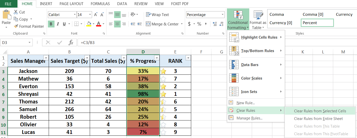
Select the group of cells from which we want to delete the conditional format ➪ Home ➪ Styles ➪ Conditional Formatting ➪ Clear Rules…➪ Clear Rules from Selected Cells.
➢ Delete All the Rules of the Current Sheet:
• Method 1: Using the Ribbon
Select the entire dataset ➪ Home ➪ Styles ➪ Conditional Formatting ➪ Clear Rules… ➪ Clear Rules from Entire Sheet.

• Method 2: Using Excel Shortcut
Select the entire dataset ➪ Press Alt+O+D (sequentially Alt, O, D) which will open the ‘Conditional Formatting Rules Manager’ dialog box ➪ Select rule one by one and click ‘Delete Rule’ ➪ Finally, click ‘OK’ or press ‘Enter’.
(V). HOW TO CHECK EXCEL CONDITIONAL FORMATTING?
Alternatively, HOW TO FIND CONDITIONAL FORMATTING IN EXCEL?
In Excel, use the ‘Go To’ special command to check (or find) cells on a worksheet that have conditional formats. To find cells with any conditional format, click any cell in the worksheet (for ‘All’ option) or click any cell with conditional format (for ‘Same’ option).
• Method 1: Using Excel Shortcut Ctrl+G or press F5 Key
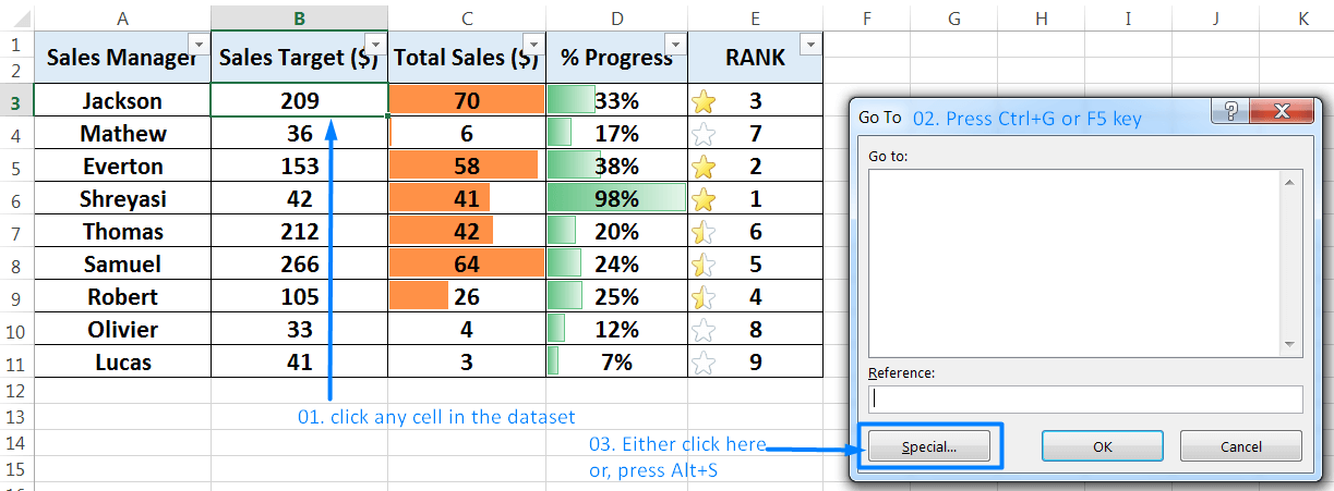
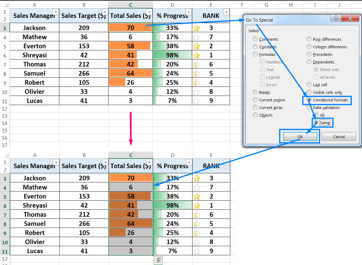
Select a cell which we want to format ➪ Press Ctrl+G or press the F5 key ➪ ‘Go To’ dialog box and click the ‘Special’ button or press Alt+S ➪ ‘Go To Special’ dialog box ➪ select the Conditional Formats ➪ To select all cells on the worksheet containing conditional formatting, select the ‘All’ option below Data Validation.

To select only the cells that contain the same conditional formatting as the active cell, select the ‘Same’ option ➪ Click ‘OK’ or press ‘Enter’.
• Method 2: Using Excel Ribbon
Choose Home ➪ Editing ➪ Find & Select ➪ ‘Go To Special’ dialog box ➪ select the Conditional Formats ➪ To select all cells on the worksheet containing conditional formatting, select the ‘All’ option below Data Validation.
To select only the cells that contain the same conditional formatting as the active cell, select the ‘Same’ option ➪ Click ‘OK’ or press ‘Enter’.
(VI). HOW TO USE EXCEL CONDITIONAL FORMATTING FORMULA?
Alternatively, HOW TO USE IF FORMULA IN CONDITIONAL FORMATTING IN EXCEL?
➢ EXAMPLE-1: APPLYING MULTIPLE NUMERIC CRITERIA
Suppose we want to format uptime (in percentage) based on the different criteria.
- Criteria1: >=99.50 (to be colored by Deep Green)
- Criteria2: >=99.30 & < 99.50 (to be colored by light Green)
- Criteria3: >=99.00 & < 99.30 (to be colored by yellow)
- Criteria4: <99.00 (to be colored by red)
We can use a formula to create a conditional formatting rule to complete the task.
Set the Criteria1: >=99.50
(i) Select a cell (i.e., A3) of the desired data range (i.e., A3:G20).
(ii) Press Alt+O+D (sequentially press Alt, O, D) which will open ‘Conditional Formatting Rules Manager’.
Or, Home ➪ Styles ➪ Conditional Formatting ➪ Manage Rules… which will open the ‘Conditional Formatting Rules Manager’ dialog box.
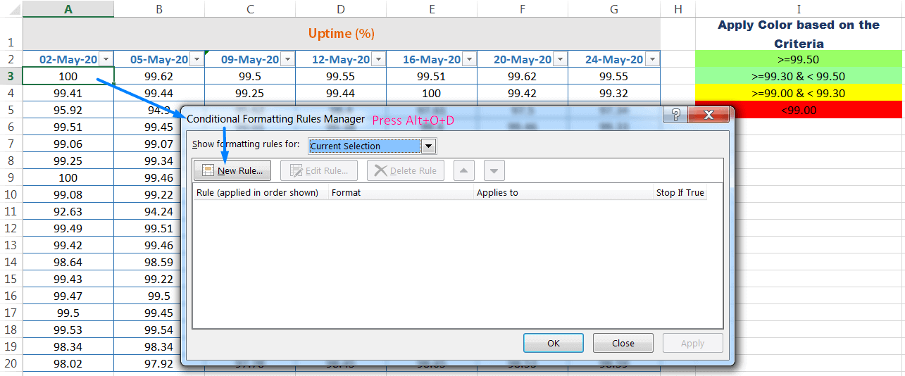
(iii) Click on ‘New Rule’ or press Alt+N which will open the ‘New Formatting Rule’ dialog box.
(iv) Select the last option ‘Use a formula to determine which cells to format’ and type the formula, using cell reference, in the ‘Format values where this formula is true:’ box.
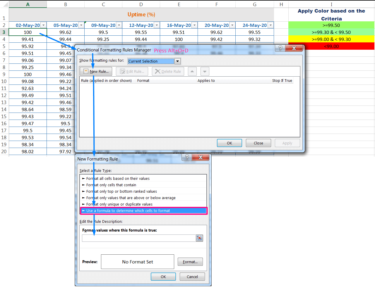
Place an equality sign (=) and select the first cell (i.e., A3) of the desired range as a cell reference. By default cell reference is the absolute cell reference (i.e., $A$3) and immediately changes it to relative cell reference (i.e., A3) by pressing the F4 key three times.
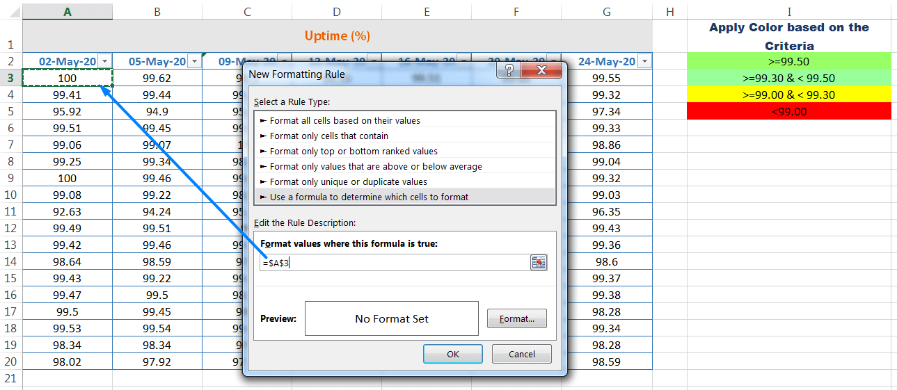
Then place the criteria >=99.50 (greater than or equal to 99.50).
Finally, it seems to be: =A3>=99.5
Then click on the ‘Format…’ tab ➪ go to the ‘Fill’ tab in the ‘Format Cells’ dialog box. Either choose a color from the palette or select ‘More Colors…’ ➪ again a ‘Colors’ dialog box opens. Choose deep green color in the ‘Standard’ tab or we can modify the density of color in the ‘Custom’ tab ➪ Click ‘OK’ to close the ‘Colors’ dialog box, again click ‘OK’ to close the ‘Format Cells’ dialog box, again click ‘OK’ to close the ‘New Formatting Rule’ dialog box.
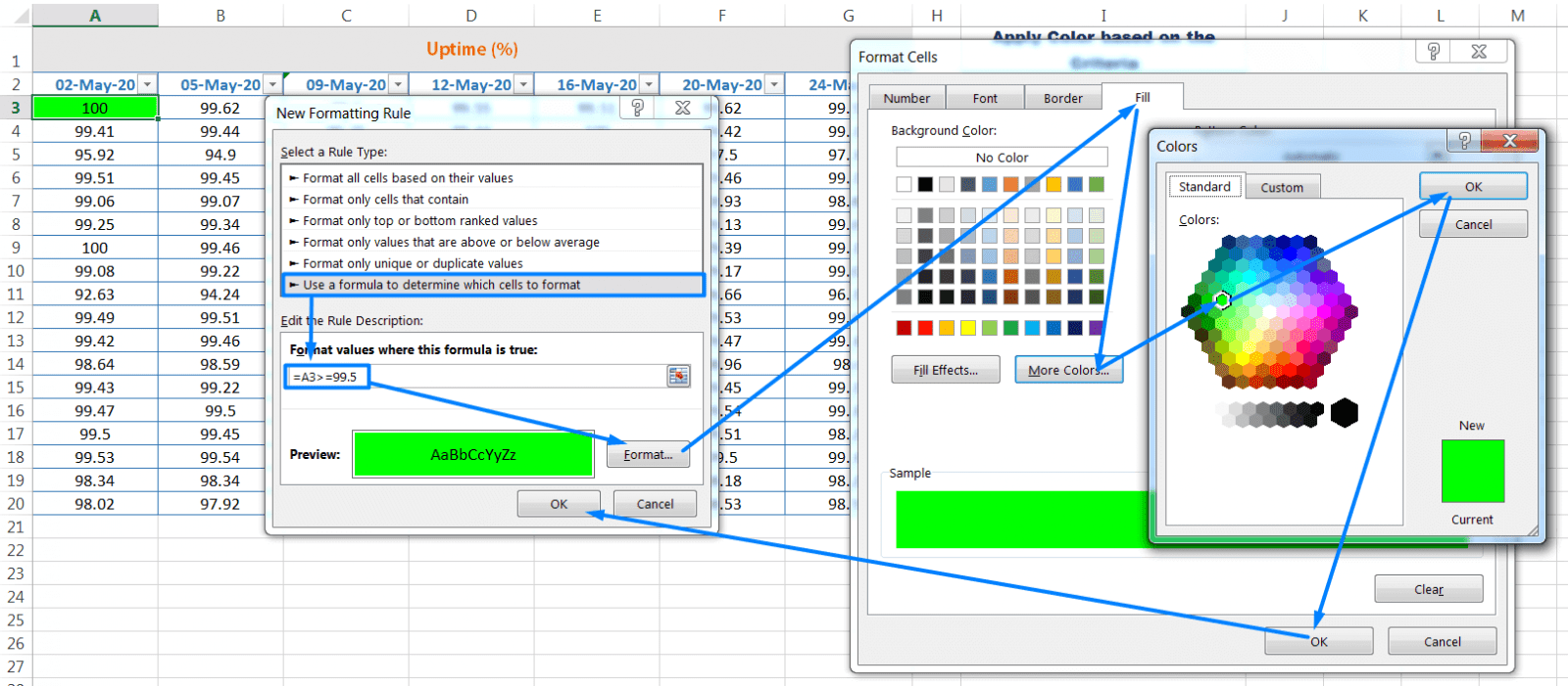
(v) Then click on ‘Apply’ to save the created first rule in the ‘Conditional Formatting Rules Manager’ dialog box.
Set the Criteria2: >=99.30 & < 99.50
Here we use the AND function. The AND function requires that both logical tests be met to apply the conditional formatting. A minimum of two logical tests is required; however, we can include additional logical tests. Note that all logical tests must be true to apply the conditional formatting.

(i) First, click on the ‘New Rule’ button or press Alt+N which will open the ‘New Formatting Rule’ dialog box.
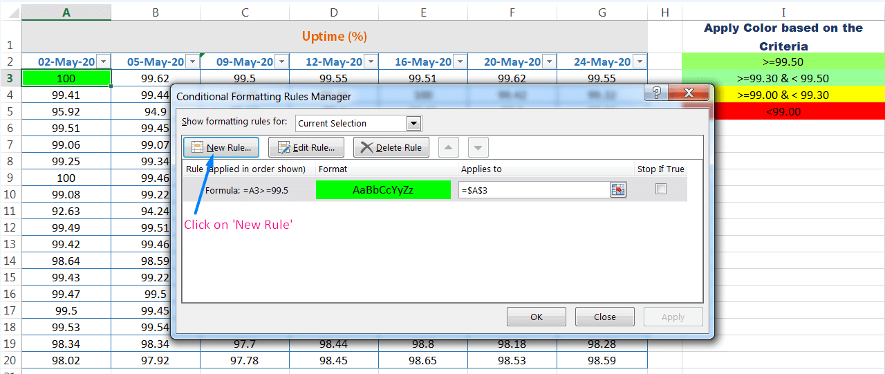
(ii) Select the last option ‘Use a formula to determine which cells to format’ and type the formula in the ‘Format values where this formula is true:’ box.
Place an equality sign (=) and type the formula =AND(A3>=99.3, A3<99.5)
Then click on the ‘Format…’ tab ➪ go to the ‘Fill’ tab in the ‘Format Cells’ dialog box. Either choose a color from the palette or select ‘More Colors…’ ➪ again a ‘Colors’ dialog box opens. Choose light green color in the ‘Standard’ tab or we can modify the density of color in the ‘Custom’ tab ➪ Click ‘OK’ to close the ‘Colors’ dialog box, again click ‘OK’ to close the ‘Format Cells’ dialog box, again click ‘OK’ to close the ‘New Formatting Rule’ dialog box.

(iii) Then click on ‘Apply’ to save the created second rule in the ‘Conditional Formatting Rules Manager’ dialog box.
Set the Criteria3: >=99.00 & < 99.30
(i) Again, click on the ‘New Rule’ button or press Alt+N which will open the ‘New Formatting Rule’ dialog box.
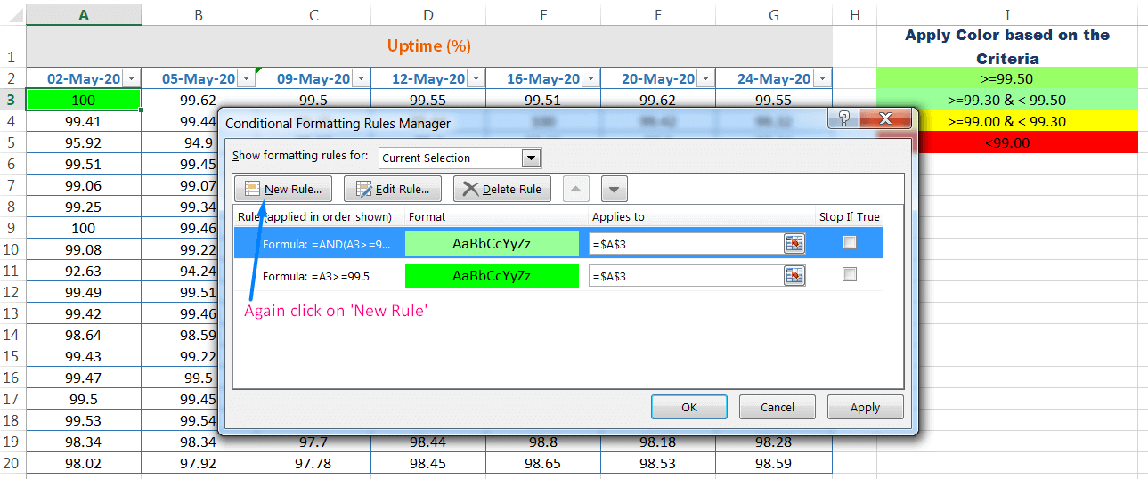
(ii) Select the last option ‘Use a formula to determine which cells to format’ and type the formula in the ‘Format values where this formula is true:’ box.
Place an equality sign (=) and type the formula =AND(A3>=99, A3<99.30)
Then click on the ‘Format…’ tab ➪ go to the ‘Fill’ tab in the ‘Format Cells’ dialog box. Either choose a color from the palette or select ‘More Colors…’ ➪ again a ‘Colors’ dialog box opens. Choose yellow color in the ‘Standard’ tab or we can modify the density of color in the ‘Custom’ tab ➪ Click ‘OK’ to close the ‘Colors’ dialog box, again click ‘OK’ to close the ‘Format Cells’ dialog box, again click ‘OK’ to close the ‘New Formatting Rule’ dialog box.

(iii) Then click on ‘Apply’ to save the created third rule in the ‘Conditional Formatting Rules Manager’ dialog box.
Set the Criteria4: < 99.00
(i) Further click on the ‘New Rule’ button or press Alt+N which will open the ‘New Formatting Rule’ dialog box.
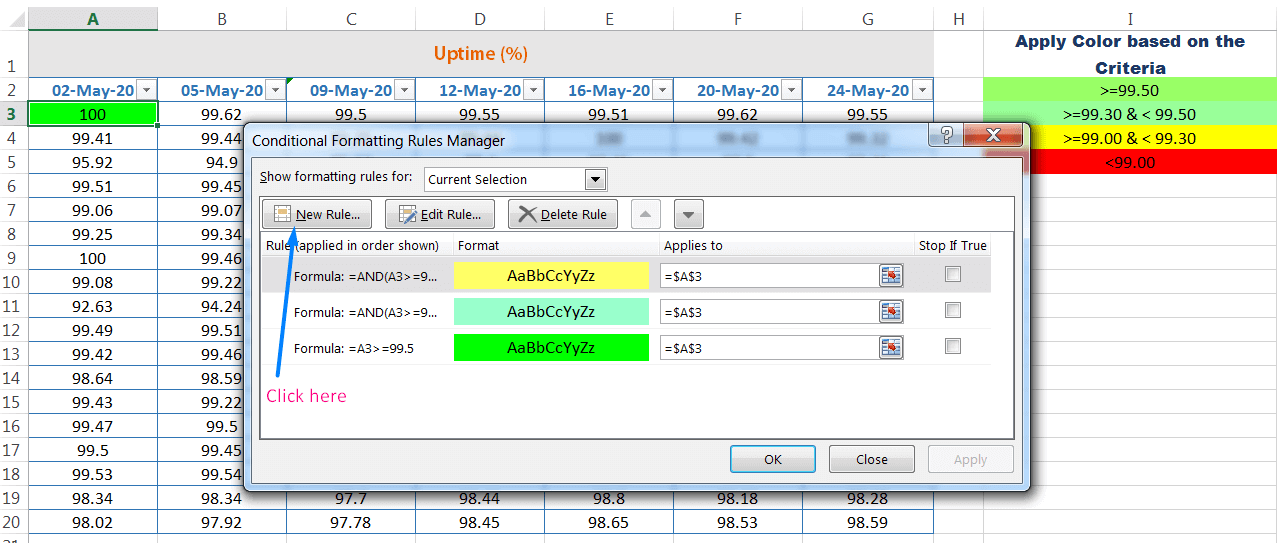
(ii) Select the last option ‘Use a formula to determine which cells to format’ and type the formula in the ‘Format values where this formula is true:’ box.
Place an equality sign (=) and type the formula =A3<99
Then click on the ‘Format…’ tab ➪ go to the ‘Fill’ tab in the ‘Format Cells’ dialog box. Choose the red color from the palette ➪ Click ‘OK’ to close the ‘Format Cells’ dialog box, again click ‘OK’ to close the ‘New Formatting Rule’ dialog box.
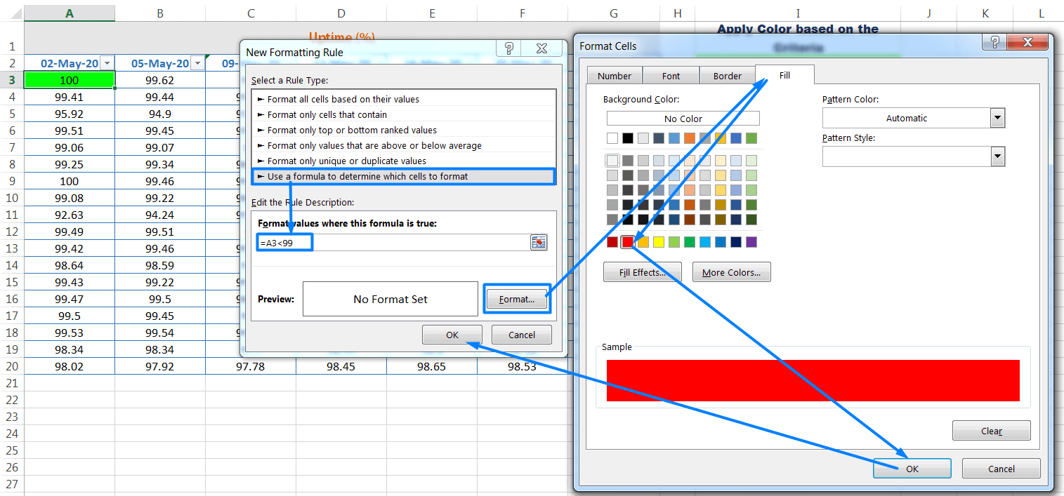
(iii) Then click on ‘Apply’ to save the created fourth rule in the ‘Conditional Formatting Rules Manager’ dialog box. Finally, press ‘OK’ to apply the conditional formats in cell A3.
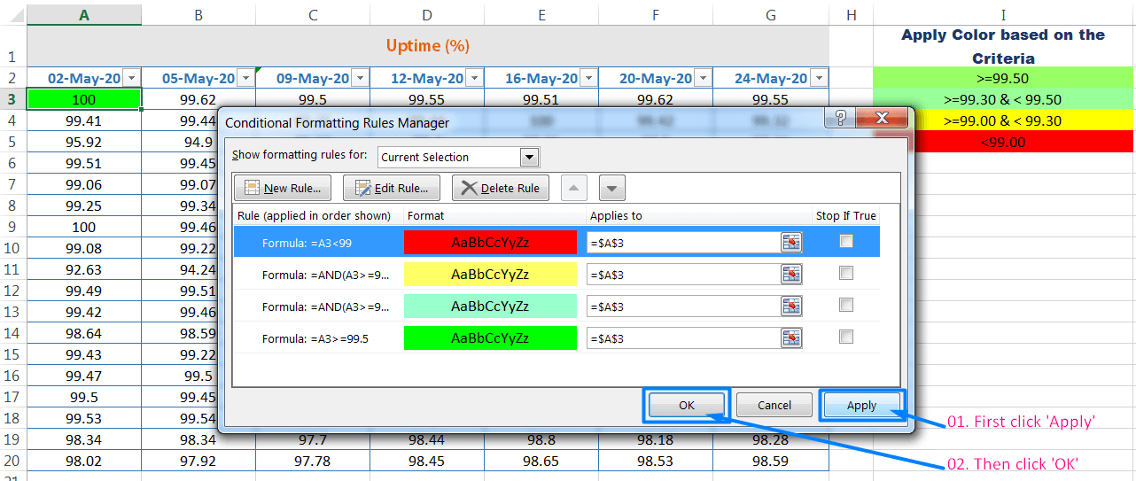
➪ HOW TO APPLY CONDITIONAL FORMATTING TO MULTIPLE CELLS?
Similar to standard formatting, Conditional formatting information is also stored in a cell. As a result, while copying a cell that contains conditional formatting, the conditional formatting also copied.
If we insert rows or columns within a range that contains conditional formatting, the new cells have the same conditional formatting.
• Method 1: Using Excel Shortcut Alt+E+S+T / Alt+Ctrl+V+T

To copy only the formatting (including conditional formatting), first, we copy the cell (i.e., A3) with Excel shortcut Ctrl+C ➪ making a selection of the entire ranges (A3:G20) where we want to apply the conditional formatting with Shift+ Right arrow (➡), Down arrow (⬇) ➪ press sequentially Alt+E+S+T (such as Alt, E, S, T) or Alt+Ctrl+V+T (such as Alt+Ctrl+V, T) which will select the ‘Formats‘option in the ‘Paste Special’ dialog box ➪ click ‘OK’ or press ‘Enter’ to accept the conditional format.
• Method 2: Using Excel Ribbon
Copy the cell (i.e., A3) ➪ making a selection of the entire ranges (A3:G20) ➪ Home ➪ Clipboard ➪ Paste drop-down ➪ Paste Special ➪ Formats ➪ to click ‘OK’ or press ‘Enter’.
As a result, conditional formatting is applied to the entire selected range.

Note: After applying conditional formats in the entire ranges, press the ‘Esc‘ (Escape) key which removes the animated marquee from the cell.
➢ EXAMPLE-2: CREATING ALTERNATE-ROW SHADING
The conditional formatting formula was applied to the range A1:D18, as shown in below Figure, to apply shading to alternate rows:
=MOD(ROW(),2)=0
How Formula Works:
Alternate row shading can make our spreadsheets easier to read. If you add or delete rows within the conditional formatting area, the shading is updated automatically.
This formula uses the ROW function (which returns the row number) and the MOD function (which returns the remainder of its first argument divided by its second argument).
 |  |
For cells in even-numbered rows, the MOD function returns 0, and cells in that row are formatted.
Steps to Start:
(i) Select the desired data range (i.e., A3:G20).
(ii) Press Alt+O+D (sequentially press Alt, O, D) which will open ‘Conditional Formatting Rules Manager’.
Or, Home ➪ Styles ➪ Conditional Formatting ➪ Manage Rules… which will open the ‘Conditional Formatting Rules Manager’ dialog box.
(iii) Further click on the ‘New Rule’ button or press Alt+N which will open the ‘New Formatting Rule’ dialog box.
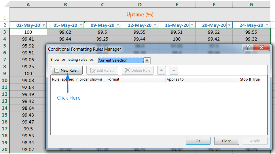
(iv) Select the last option ‘Use a formula to determine which cells to format’ and type the formula in the ‘Format values where this formula is true:’ box.
Place an equality sign (=) and type the formula =MOD(ROW(),2)=0
Then click on the ‘Format…’ tab ➪ go to the ‘Fill’ tab in the ‘Format Cells’ dialog box. Either choose a color from the palette or select ‘More Colors…’ ➪ again a ‘Colors’ dialog box opens. Choose any color in the ‘Custom’ tab and we can modify the density of color in the ‘Custom’ tab ➪ Click ‘OK’ to close the ‘Colors’ dialog box, again click ‘OK’ to close the ‘Format Cells’ dialog box, again click ‘OK’ to close the ‘New Formatting Rule’ dialog box.

(v) Then click on ‘Apply’ to save the created rule in the ‘Conditional Formatting Rules Manager’ dialog box. Finally, press ‘OK’ to apply the conditional formats (Alternate-Row Shading) to the entire range.
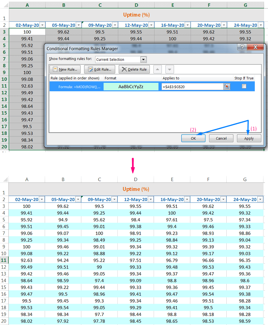
➢ EXAMPLE-3: CREATING ALTERNATE-COLUMN SHADING
For alternate shading of columns, use the COLUMN function instead of the ROW function.
=MOD(COLUMN(),2)=0
Steps to Start:
(i) Select the desired data range (i.e., A3:G20).
(ii) Press Alt+O+D (sequentially press Alt, O, D) which will open ‘Conditional Formatting Rules Manager’.
Or, Home ➪ Styles ➪ Conditional Formatting ➪ Manage Rules… which will open the ‘Conditional Formatting Rules Manager’ dialog box.
(iii) Further click on the ‘New Rule’ button or press Alt+N which will open the ‘New Formatting Rule’ dialog box.
Or, Home ➪ Styles ➪ Conditional Formatting ➪ New Rule
(iv) Select the last option ‘Use a formula to determine which cells to format’ and type the formula in the ‘Format values where this formula is true:’ box.
Place an equality sign (=) and type the formula =MOD(COLUMN(),2)=0
Then click on the ‘Format…’ tab ➪ go to the ‘Fill’ tab in the ‘Format Cells’ dialog box. Choose any color from the palette ➪ Click ‘OK’ to close the ‘Format Cells’ dialog box, again click ‘OK’ to close the ‘New Formatting Rule’ dialog box.
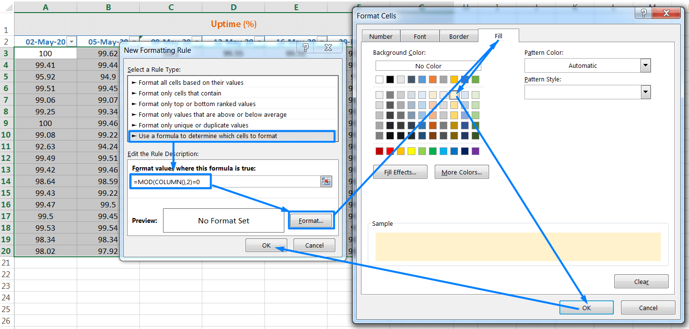
(v) Then click on ‘Apply’ to save the created rule in the ‘Conditional Formatting Rules Manager’ dialog box. Finally, press ‘OK’ to apply the conditional formats (Alternate-Column Shading) to the entire range.

➢ EXAMPLE-4: CREATING CHECKERBOARD SHADING
The following formula is a variation on the example in the preceding section. It applies formatting to alternate rows and columns, creating a checkerboard effect:
=MOD(ROW(),2)=MOD(COLUMN(),2)
Steps to Start:
(i) Select the desired data range (i.e., A3:G20).
(ii) Press Alt+O+D (sequentially press Alt, O, D) which will open ‘Conditional Formatting Rules Manager’.
Or, Home ➪ Styles ➪ Conditional Formatting ➪ Manage Rules… which will open the ‘Conditional Formatting Rules Manager’ dialog box.
(iii) Further click on the ‘New Rule’ button or press Alt+N which will open the ‘New Formatting Rule’ dialog box.
Or, Home ➪ Styles ➪ Conditional Formatting ➪ New Rule
(iv) Select the last option ‘Use a formula to determine which cells to format’ and type the formula in the ‘Format values where this formula is true:’ box.
Place an equality sign (=) and type the formula =MOD(ROW(),2)=MOD(COLUMN(),2)

Then click on the ‘Format…’ tab ➪ go to the ‘Fill’ tab in the ‘Format Cells’ dialog box. Either choose a color from the palette or select ‘More Colors…’ ➪ again a ‘Colors’ dialog box opens. Choose any color in the ‘Standard’ tab or we can modify the density of color in the ‘Custom’ tab ➪ Click ‘OK’ to close the ‘Colors’ dialog box, again click ‘OK’ to close the ‘Format Cells’ dialog box, again click ‘OK’ to close the ‘New Formatting Rule’ dialog box.
(v) Then click on ‘Apply’ to save the created rule in the ‘Conditional Formatting Rules Manager’ dialog box. Finally, press ‘OK’ to apply the conditional formats (Creating Checkerboard Shading) to the entire range.

Shading Groups of Rows
Here’s another row shading variation. The following formula shades alternate groups of rows. It produces four shaded rows, followed by four unshaded rows, followed by four more shaded rows, and so on:
=MOD(INT((ROW()-1)/4)+1,2)=1
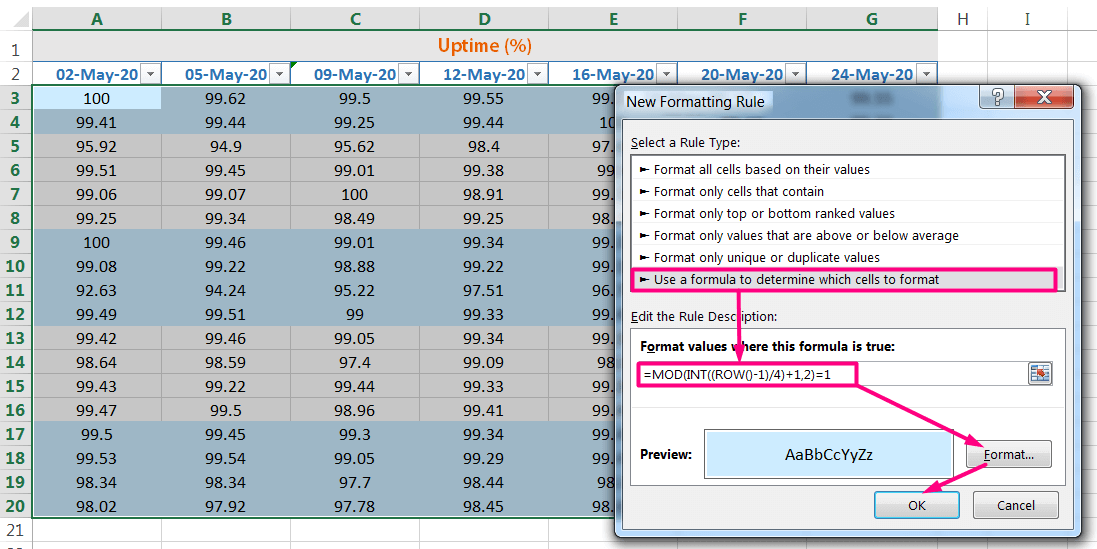
For the different sized groups, change the 4 to some other value. For example, use this formula to shade alternate groups of three rows:
=MOD(INT((ROW()-1)/3)+1,2)=1
➢ EXAMPLE-5: HIGHLIGHTING A ROW BASED ON VALUE (TEXT)
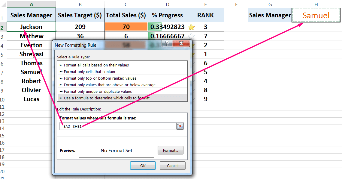
The below figure shows a worksheet that contains a conditional formula in the range A2:E10.
If a name entered in cell H1 is found in the first column, the entire row for that name is highlighted.
The conditional formatting formula is =$A2=$H$1
Notice that a mixed reference is used for cell A3, where the column part of the reference is absolute, but the row is relative, the comparison is always done using the contents of column A. Otherwise, it only formats the column A based on the matched value.
Steps to Start:
(i) First, we select cell A2 in the desired data range (i.e., A1:E10) ➪ then Press Alt+O+D (sequentially press Alt, O, D) which will open ‘Conditional Formatting Rules Manager’.
Or, Home ➪ Styles ➪ Conditional Formatting ➪ Manage Rules… which will open the ‘Conditional Formatting Rules Manager’ dialog box.
(ii) Further click on the ‘New Rule’ button or press Alt+N which will open the ‘New Formatting Rule’ dialog box.
Or, Home ➪ Styles ➪ Conditional Formatting ➪ New Rule

(iii) Select the last option ‘Use a formula to determine which cells to format’ and type the formula in the ‘Format values where this formula is true:’ box.
Type the conditional formatting formula in the box: =$A2=$H$1
Please note that we should convert the cell reference A2 from the absolute to the mixed cell reference, where columns being fixed (e.g., $A$2 ➪ $A2) by pressing the F4 key twice. So in that case, while we copying the formula vertically (column-wise), the column addresses remain fixed, but row numbers simultaneously changed, like $A2, $A3, $A4, $A5…so on.

Whereas cell H1 refers to a specific value, either text string or numeric value, for example, ‘Samuel‘, based on which conditional formats applied to the entire range. So, H1 should be absolute (i.e., $H$1), which means while we copying the formula horizontally (row-wise) or vertically (column-wise) in any direction, columns address, and row number do not change at all.
(iv) Then click on the ‘Format…’ tab ➪ go to the ‘Fill’ tab in the ‘Format Cells’ dialog box. Either choose a color from the palette or select ‘More Colors…’ ➪ again a ‘Colors’ dialog box opens. Choose any color in the ‘Standard’ tab or we can modify the density of color in the ‘Custom’ tab ➪ Click ‘OK’ to close the ‘Colors’ dialog box, again click ‘OK’ to close the ‘Format Cells’ dialog box, again click ‘OK’ to close the ‘New Formatting Rule’ dialog box.
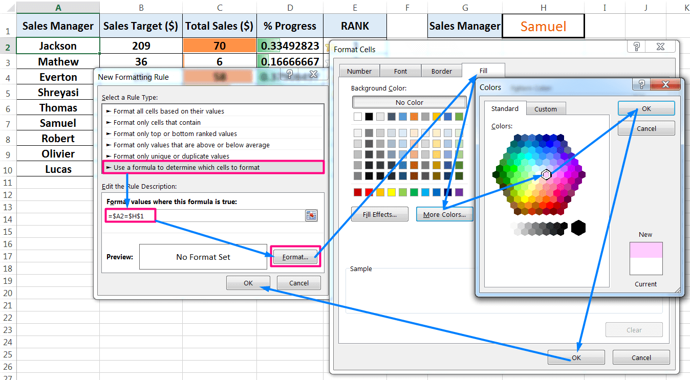
(v) Then click on ‘Apply’ to save the created rule in the ‘Conditional Formatting Rules Manager’ dialog box. Finally, press ‘OK’ to apply the conditional formatting to a specific cell (i.e., A3).

(vi) Applying Conditional Formats from a Cell to the Entire Range:
Copy the cell A2 with Excel shortcut Ctrl+C ➪ making a selection to the entire range with Shift + Right arrow (➡), Down arrow (⬇) ➪ press Alt+E+S+T (sequentially press Alt, E, S, T) or Alt+Ctrl+V+T (sequentially press Alt+Ctrl+V, T) which will select the option ‘Formats‘ in the ‘Paste Special’ dialog box ➪ Click ‘OK’ or press ‘Enter’ to accept the conditional formats.

Finally, get the result (conditional formatting based on value or text) across the entire selection.

➢ EXAMPLE-6: IDENTIFYING TEXT CELLS THAT BEGIN WITH SPECIFIED LETTERS
Identifying text cells that begin with specified letters
The worksheet shown in the below Figure contains a list of names in the range A1:E10. Cell H1 contains one or more letters of the alphabet. A conditional formatting formula highlights the names that begin with the letter sequence in cell H1.
Here we use the LEFT function along with the LEN function.
➢ The LEFT Function
The syntax for the LEFT function is:

Arguments are
• text is either text or a cell address containing the text
• num_chars is the number of characters we want from the beginning of the string.
➢The LEN Function
We can use the LEN function to count the number of characters in a text value.

For example, the string Shreyasi contains 8 characters.
Steps to Start:
(i) First, we select cell A2 in the desired data range (i.e., A1:E10) ➪ then Press Alt+O+D (sequentially press Alt, O, D) which will open ‘Conditional Formatting Rules Manager’.
Or, Home ➪ Styles ➪ Conditional Formatting ➪ Manage Rules… which will open the ‘Conditional Formatting Rules Manager’ dialog box.
(ii) Further click on the ‘New Rule’ button or press Alt+N which will open the ‘New Formatting Rule’ dialog box.
Or, Home ➪ Styles ➪ Conditional Formatting ➪ New Rule
(iii) Select the last option ‘Use a formula to determine which cells to format’ and type the formula in the ‘Format values where this formula is true:’ box.
Type the conditional formatting formula in the box: =LEFT(A2,LEN($H$1))= $H$1
Please note that we should convert the cell reference A2 from the absolute to the relative cell reference (e.g., $A$2 ➪ A2) by pressing the F4 key thrice. As a result, we can apply the same formatting to the entire range.
Whereas cell H1 refers to a specific character ‘Sh‘, based on which conditional formats applied to the entire range. So, H1 should be absolute (i.e., $H$1), which means while we copying the formula horizontally (row-wise) or vertically (column-wise) in any direction, columns address, and row number do not change at all.
Then click on the ‘Format…’ tab ➪ go to the ‘Fill’ tab in the ‘Format Cells’ dialog box. Choose any color from the palette ➪ Click ‘OK’ to close the ‘Format Cells’ dialog box, again click ‘OK’ to close the ‘New Formatting Rule’ dialog box.
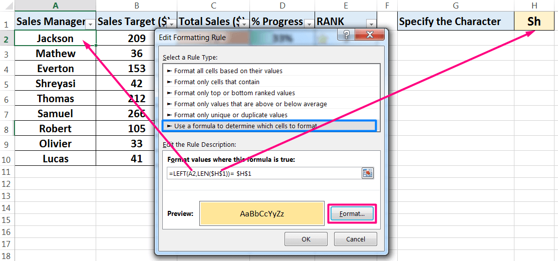
(iv) Then click on ‘Apply’ to save the created rule in the ‘Conditional Formatting Rules Manager’ dialog box. Finally, press ‘OK’ to apply the conditional formatting to a specific cell (i.e., A3).
(v) Applying Conditional Formats from a Cell to the Entire Range:
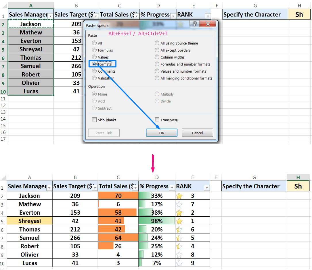
Copy the cell A3 with Excel shortcut Ctrl+C ➪ making a selection to the entire range with Shift + Right arrow (➡), Down arrow (⬇) ➪ press Alt+E+S+T (sequentially press Alt, E, S, T) or Alt+Ctrl+V+T (sequentially press Alt+Ctrl+V, T) which will select the option ‘Formats‘ in the ‘Paste Special’ dialog box ➪ Click ‘OK’ or press ‘Enter’ to accept the conditional formats.
➢ EXAMPLE-7: IDENTIFYING CELLS THAT MEET NUMERIC CRITERIA
The example in this section is similar to the previous example, but it involves values. The range A3:G20 uses the following conditional formatting formula:
=COUNTIF(A3,$J$1)=1
This formula takes advantage of the fact that the COUNTIF function can handle the criteria that are entered in a cell.
Steps to Start:
(i) First, select a cell A3 in the desired data range (i.e., A2:G20).
(ii) Press Alt+O+D (sequentially press Alt, O, D) which will open ‘Conditional Formatting Rules Manager’.
Or, Home ➪ Styles ➪ Conditional Formatting ➪ Manage Rules… which will open the ‘Conditional Formatting Rules Manager’ dialog box.
(iii) Further click on the ‘New Rule’ button or press Alt+N which will open the ‘New Formatting Rule’ dialog box.
Or, Home ➪ Styles ➪ Conditional Formatting ➪ New Rule

(iv) Select the last option ‘Use a formula to determine which cells to format’ and type the formula in the ‘Format values where this formula is true:’ box.
Place an equality sign (=) and type the formula =COUNTIF(A3,$J$1)=1
Please note that we should convert the cell reference A3 from the absolute to the relative cell reference (e.g., $A$3 ➪ A3) by pressing the F4 key thrice. As a result, we can apply the same formatting to the entire range.
Whereas cell J1 refers to a specific value 97, based on which conditional formats applied to the entire range. So, J1 should be absolute (i.e., $J$1), which means while we copying the formula horizontally (row-wise) or vertically (column-wise) in any direction, columns address, and row number do not change at all.
Then click on the ‘Format…’ tab ➪ go to the ‘Fill’ tab in the ‘Format Cells’ dialog box. Choose any color from the palette ➪ Click ‘OK’ to close the ‘Format Cells’ dialog box, again click ‘OK’ to close the ‘New Formatting Rule’ dialog box.

(v) Then click on ‘Apply’ to save the created rule in the ‘Conditional Formatting Rules Manager’ dialog box. Finally, press ‘OK’ to apply the conditional formatting to a specific cell (i.e., A3).

(vi) Applying Conditional Formats from a Cell to the Entire Range:
Copy the cell A3 with Excel shortcut Ctrl+C ➪ making a selection to the entire range with Shift + Right arrow (➡), Down arrow (⬇) ➪ press Alt+E+S+T (sequentially press Alt, E, S, T) or Alt+Ctrl+V+T (sequentially press Alt+Ctrl+V, T) which will select the option ‘Formats‘ in the ‘Paste Special’ dialog box ➪ Click ‘OK’ or press ‘Enter’ to accept the conditional formats.

Finally, get the result (conditional formatting based on numeric value) across the entire selection.

➢ EXAMPLE-8: USING EXCEL CONDITIONAL FORMATTING TO HIDE ERRORS
Sometimes the error values won’t be much of a concern to us and we may just want to hide them by using Conditional Formatting. As a result, we can render all the error values invisible.
Following is the step by step process on how we can do that:
Steps to Start:
(i) First, select a range of cells A1:A11 containing error values that we want to hide.
(ii) Press Alt+O+D (sequentially press Alt, O, D) which will open ‘Conditional Formatting Rules Manager’.
Or, Home ➪ Styles ➪ Conditional Formatting ➪ Manage Rules… which will open the ‘Conditional Formatting Rules Manager’ dialog box.
(iii) Further click on the ‘New Rule’ button or press Alt+N which will open the ‘New Formatting Rule’ dialog box.
Or, Home ➪ Styles ➪ Conditional Formatting ➪ New Rule

(iv) In the Select a Rule Type box, click the second option ‘Format only cells that contain‘.
(v) Click the ‘Cell Value‘ drop-down list and select ‘Errors‘.

(vi) Click the Format button to open the Format Cells dialog box.
(vii) Click the Color drop-down menu to open the color palette. Select White color and click OK. If the selected cells are shaded, then choose the same color in the color palette.
(viii) Click OK to close the New Formatting Rule dialog box and return to the worksheet.

(ix) Then click on ‘Apply’ to save the created rule in the ‘Conditional Formatting Rules Manager’ dialog box. Finally, press ‘OK’ to apply the conditional formatting to the specific range (i.e., A1:A11).
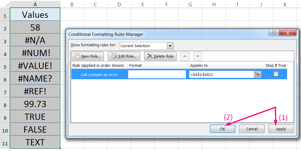
All the error values in the selected cells would have disappeared from the worksheet.


Premium Courses on ed2go
Premium Courses on Coursera
Premium Courses on Udemy

12 Examples || How to Use Excel Go To Special?
07 Points Guided You How to Find And Replace in Excel?
05 Points Should Learn How to Freeze Panes in Excel?
12 Things Guided You How to Manage An Excel Workbook
03 Useful Methods : Add Numbers With AutoSum Excel
04 Simple to Advanced Methods: How to Filter in Excel?
05 Best Ways: Create Password Protect Excel & Unprotect it
04 Alternative Methods: How to Wrap Text in Excel?
04 BEST WAYS: HOW TO TRANSPOSE DATA IN EXCEL
Tutorial 01: How to Use Excel SUMIFS Function with Single & Multiple Criteria
Thanks for your interest joining to Advance Excel Forum community.
Something went wrong.

Join Our Community List
Subscribe to our mailing list and get interesting stuff and updates to your email inbox.
* VERIFY & CONFIRM YOUR EMAIL * We respect your privacy and take protecting it seriously*.


