I. WHAT IS EXCEL AVERAGEIFS FUNCTION?

The Excel AVERAGEIFS Function is the advanced statistical category function that calculates the average (arithmetic mean) of a range of cells that meet the multiple criteria. Thus, we can select multiple ranges and specify a different criterion for each range. We can enter up to 127 criteria ranges and criteria arguments at a time in the AVERAGEIFS function.

Whereas the Excel AVERAGEIF function calculates the average (arithmetic mean) of a range of cells that meet a single criterion.

II. FEATURES OF EXCEL AVERAGEIFS FUNCTION

(01) The Excel AVERAGEIFS function is generally used to get the average value in a range of cells based on a match of a single criterion or multiple criteria. Thus, we can select multiple ranges and specify a different criterion for each range. 

(02) Cells in a range that contain logical values like TRUE or FALSE are ignored.

(03) The Excel AVERAGEIFS function will return an error (#DIV0!) if the range is a blank or text value.

(04) If a cell in criteria is empty it is treated as a zero (0) value.

(05) AVERAGEIF returns the #DIV/0! Error value if no cells in the range meet the criteria.

(06) We can enter up to 127 criteria ranges and criteria arguments at a time in the AVERAGEIFS function.

(07) Average_range does not necessarily need to be the same number of rows and columns as criteria_range (or, the range for the AVERAGEIF function). The cells that are averaged are determined by using the top-left cell in average_range as the first cell and then including cells that match the same number of rows and columns in criteria_range (or, the range for the AVERAGEIF function). See the examples below:

• If the range is A1:A10 and the average_range is B1:B10, then the actual cells evaluated would be B1:B10.

• If the range is A1:A10 and the average_range is B1:B5, then the actual cells evaluated would be B1:B10.

• If the range is A1:B5 and the average_range is C1:C3, then the actual cells evaluated would be C1:C5.

(08) The Excel AVERAGEIFS function only follows the AND logic, which means all the criteria must be TRUE for the number in the corresponding range to be added.

(09) The Excel AVERAGEIFS function supports logical operators when criteria are numeric values (which may be an integer, decimal, date, and time).

We should use logical operators within double-quotes.

Logical operators are: “=” (equal to), “<=” (not equal to), “=” (greater than), “<” (less than),”>=” (greater than or equal to), “<=” (less than or equal to), ” ” (space or blanks).

With the help of logical operators, the Excel AVERAGEIFS function supports expression, and expression should be inside the double quotes.

For example: “>”&10; “>10”; “<=”&0; “<=0” “<>”&”” etc. 

(10) Similar to the Excel SUMIFS function, the AVERAGEIFS function supports wildcard characters (asterisk ‘*‘, question mark ‘?‘) for the partial match when criteria are text strings.

Text strings can be the name (“Apple”, “USA”, “Shreyasi”), weekdays (“Monday”, “Tuesday”, etc.,), months (“January”, “February”, etc.,).

Text criteria (i.e., non-numeric criteria) must be enclosed in double-quotes, but numeric criteria do not require any quotes.

An asterisk character (*) matches any sequence of characters, while a question mark (?) matches any one character.

(11) The Excel AVERAGEIFS function is case-insensitive, which means the upper case, proper case, and lower case are treated as identical. For example, the text strings “THOMAS”, “Thomas”, and “thomas” will be considered to be equal.

III. TYPES OF EXCEL AVERAGE FUNCTION

IV. WHAT ARE THE DIFFERENCES BETWEEN AVERAGE AND AVERAGEA?

The following figure shows the differences between the AVERAGE function and the AVERAGEA function for average in Excel and the different results they return: 

The AVERAGE function ignores any text, and logical values (TRUE and FALSE) if there are any in the selected range, whereas the AVERAGEA function evaluates them. For example, any text evaluates them as zero (0), logical values (TRUE evaluates as 1; FALSE evaluates as 0).

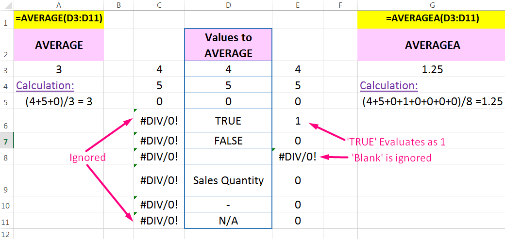
However, both the functions ignore ‘blank’ cells from the calculation. 

V. WHAT ARE THE DIFFERENCES BETWEEN AVERAGEIF AND AVERAGEIFS?

• The AVERAGEIFS function is almost the same as the AVERAGEIF function, except for one difference; and that is the allowance to add more than one criterion.

• When we want to get the average values (arithmetic mean) in a range based on a single criterion, then we can use either SUMIF or SUMIFS function. When we allow any of them, we will notice that the order of arguments is different between the AVERAGEIFS function and the AVERAGE function. 

The Average_range is the first argument in the AVERAGEIFS function, whereas the third argument in the AVERAGEIF function.

VI. WHAT ARE THE SIMILARITIES BETWEEN AVERAGEIF AND AVERAGEIFS?

• If Average_range is omitted from the function argument, the range (for AVERAGEIF) or the criteria_range (for AVERAGEIFS) is used. 

• If a cell in Average_range is an empty cell, both AVERAGEIF and AVERAGEIFS ignore it.

• If the entire range is blank or contains text values, both AVERAGEIF and AVERAGEIFS return the #DIV/0! error value.

• If no cells in the range meet the criteria, both AVERAGEIF and AVERAGEIFS return the #DIV/0! error value. 

VII. EXAMPLES OF EXCEL AVERAGEIFS FUNCTION

(01) Ignore ‘Blanks’ and ‘Zero’ Values from Average by Using Excel AVERAGEIFS Function

In this example, we have a list of sales quantities of different Sales Managers for several days. We want to find the average sales per Sales Manager for entries that ignore ‘Blanks‘ and ‘Zero‘ values.

■ Steps to Start:

(i) Applying Excel AVERAGEIFS Function in a Separate Cell:

Place an equality sign (=) in cell J3 and type ‘aver…’, select the AVERAGEIFS function from the below suggestion list of Down Arrow key (⬇), and press the ‘Tab’ key. The AVERAGEIFS syntax appears with an open parenthesis.

Note: the upper or lower case does not matter in syntax, Excel by default considers it in upper case.

We apply the following formula to solve the problem:

=AVERAGEIFS(C3:I3, C3:I3, “<>”&0, C3:I3, “<>”&””)

• The average_range argument references the range C3:I3. This is the range for which we want to calculate the average.

• The criteria_range1 is C3:I3, the same as average_range, and from where the AVERAGEIFS formula ignores the zero values.

• The criteria1 argument is “<>”&0, which refers not equal to zero. ‘Not equal to’ symbol must be quoted in a double quotation mark, whereas it does not need for numeric values. An ampersand symbol (&) makes a bridge between them.   

• The criteria_range2 is C3:I3, the same as average_range and criteria_range1, and from where the AVERAGEIFS formula ignores the blank cells.

• The criteria2 argument is “<>”&””, which refers not equal to blanks. Similarly, the ‘Not equal to’ symbol must be quoted in a double quotation mark, whereas it does not require space (” “). An ampersand symbol (&) makes a bridge between them.

Either we close the last parenthesis and press ‘Enter‘ to accept the formula, or before closing the last parenthesis if we press ‘Enter’, Excel by default closes the last parenthesis as well.  

(ii) Applying Cell References:

• Select the average_range C3:I3 and press the F4 key thrice which will convert the range from the relative cell reference to the mixed cell reference (where the absolute column, but the relative row). So, the range is converted from C3:I3 ➪ $C3:$I3. As a result, if the formula copies downward, the column addresses (C to I) remain fixed but the row numbers simultaneously changed.   

• Similarly, select and convert the criteria_range1 and criteria_range2 to the mixed cell reference (where the absolute column, but the relative row) by pressing the F4 key thrice. As a result, the range is converted from C3:I3 ➪ $C3:$I3

When the formula is copied vertically (column-wise), the column addresses remain fixed, but the row number changes accordingly.

=AVERAGEIFS($C3:$I3, $C3:$I3, “<>”&0, $C3:$I3, “<>”&””)

Press Enter to apply the formula. If the last parenthesis will close automatically if we do not close it.

Must Read: 03 Types of Excel Cell Reference: Relative, Absolute & Mixed

(iii) Extending the Formula Till the End of the Range ➢ Alt+E+S+R / Alt+Ctrl+V+R

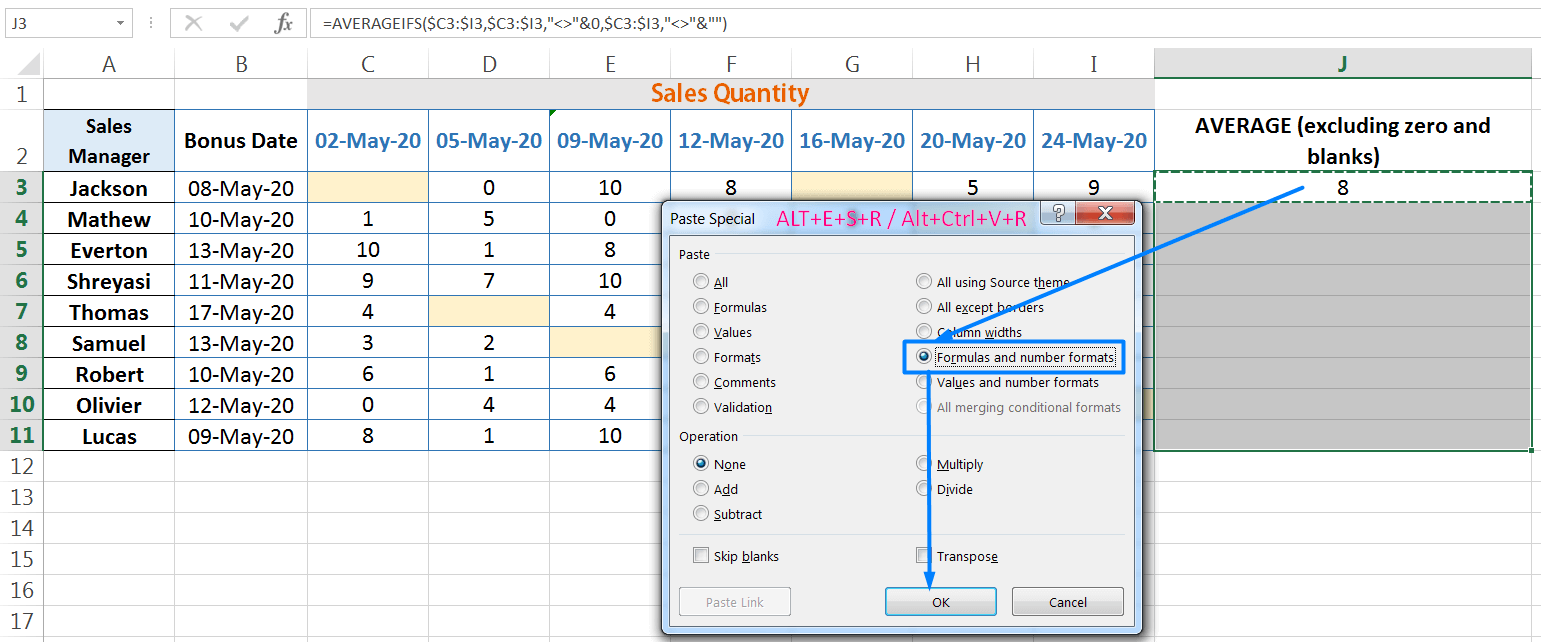
Copy the cell J3 with Excel shortcut Ctrl+C ➪ Making a selection of the entire ranges with Shift+ Right arrow (➡),  Down arrow (⬇) ➪ After copied the cell, press Alt+E+S+R ( sequentially press Alt, E, S, R) or press Alt+Ctrl+V+R (hold Alt+Ctrl+V, then press R) which will select the option ‘Formulas and number formats‘ in the ‘Paste Special’ dialog box ➪ Finally, click ‘OK’ or press ‘Enter’ from the keyboard to accept the formula.

As a result, the formula will be copied till the end of the range without copying the cell formatting.

Must Read: Paste Special in Excel Vs Break Link – Which one is Better?

(02) To Calculate Average Sales in Between Two Criteria by Using Excel AVERAGEIFS Function

In this example, we have a list of sales quantities of different Sales Managers for several days. We want to find the average sales per Sales Manager for entries that meet certain criteria. In this case, we’ve considered the value range between >=5 (greater than or equal to 5) and <=10 (less than or equal to 10). 

■ Steps to Start:

(i) Applying Excel AVERAGEIFS Function in a Separate Cell:

Place an equality sign (=) in cell J3 and apply the following Excel AVERAGEIFS formula to solve the problem:

=AVERAGEIFS(C3:I3, C3:I3, “>=”&5, C3:I3, “<=”&10)

• The average_range argument references the range C3:I3. This is the range for which we want to calculate the average.

• The criteria_range1 is C3:I3, the same as average_range, and from where the AVERAGEIFS formula calculates the first criteria (i.e., “>=”&5) from the same range.  

• The criteria1 argument is “>=”&5, which refers to greater than or equal to 5. ‘Greater than or equal to’ symbol must be quoted in a double quotation mark, whereas it does not need for numeric values. An ampersand symbol (&) makes a bridge between them.   

• The criteria_range2 is C3:I3, the same as average_range and criteria_range1, and from where the AVERAGEIFS formula calculates the second criteria (i.e., “<=”&10) from the same range.  

• The criteria2 argument is “<=”&10, which refers to less than or equal to 10. Similarly, the ‘less than or equal to’ symbol must be quoted in a double quotation mark. An ampersand symbol (&) makes a bridge between them.

Either we close the last parenthesis and press ‘Enter‘ to accept the formula, or before closing the last parenthesis if we press ‘Enter’, Excel by default closes the last parenthesis as well.

(ii) Applying Cell References:

• Select the average_range C3:I3 and press the F4 key thrice which will convert the range from the relative cell reference to the mixed cell reference (where the absolute column, but the relative row). So, the range is converted from C3:I3 ➪ $C3:$I3. As a result, if the formula copies downward, the column addresses (C to I) remain fixed but the row numbers simultaneously changed.

• Similarly, select and convert the criteria_range1 and criteria_range2 to the mixed cell reference (where the absolute column, but the relative row) by pressing the F4 key thrice. As a result, the range is converted from C3:I3 ➪ $C3:$I3

When the formula is copied vertically (column-wise), the column addresses remain fixed, but the row number changes accordingly.

=AVERAGEIFS($C3:$I3, $C3:$I3, “>=”&5, $C3:$I3, “<=”&10)

Press Enter to apply the formula. If the last parenthesis will close automatically if we do not close it.

(iii) Extending the Formula Till the End of the Range ➢ Alt+E+S+R / Alt+Ctrl+V+R

Copy the cell J3 with Excel shortcut Ctrl+C ➪ Making a selection of the entire ranges with Shift+ Right arrow (➡),  Down arrow (⬇) ➪ After copied the cell, press Alt+E+S+R ( sequentially press Alt, E, S, R) or press Alt+Ctrl+V+R (hold Alt+Ctrl+V, then press R) which will select the option ‘Formulas and number formats‘ in the ‘Paste Special’ dialog box ➪ Finally, click ‘OK’ or press ‘Enter’ from the keyboard to accept the formula.

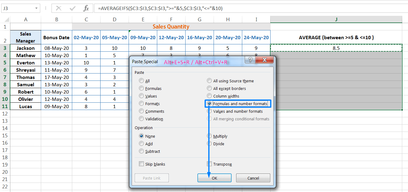
As a result, the formula will be copied till the end of the range without copying the cell formatting.

(03) To Calculate Average Sales Pre- and Post from Bonus Date by Using Excel AVERAGEIFS Function

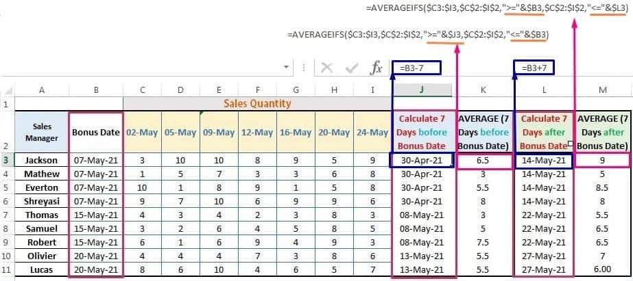
In the below example, we try to calculate an average sales pre-and post- seven days from the Bonus Date.

We find Bonus Dates in column B. Based on the Bonus Date, we calculate the 07 days pre-sales average and the 07 days post-sales average of the individual Sales Manager.  

In this case, we separately calculate pre-and-post Bonus Dates in column J and column L, respectively. 

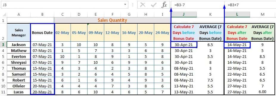
■ To Calculate Date 7 Days Before The Bonus Date:

In cell J3, we put a formula =B3-7. The value in cell J3 is always less than the value in cell B3. This concept is applied in the AVERAGEIFS formula. 

■ To Calculate Date 7 Days After The Bonus Date:

In cell L3, we put a formula =B3+7. The value in cell L3 is always greater than the value in cell B3. Similarly, this concept is applied in the AVERAGEIFS formula. 

■ To Calculate Average Sales 7 Days Before The Bonus Date:

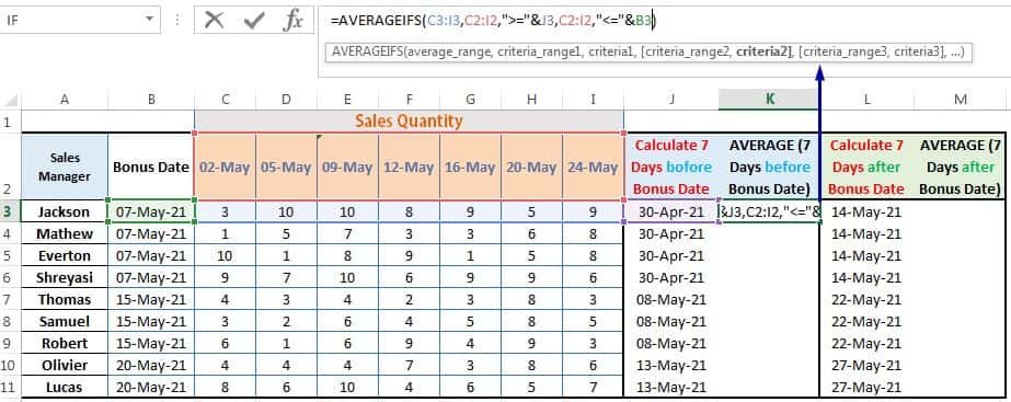
In cell K3, we put the following AVERAGEIFS formula 

=AVERAGEIFS(C3:I3, C2:I2, “>=”&J3, C2:I2, “<=”&B3)

• The average_range argument references the range C3:I3. This is the range for which we want to calculate the average.

• The criteria_range1 is C2:I2, the date of the sales range and from where the AVERAGEIFS formula calculates the first criteria (i.e., criteria1). 

• The criteria1 argument is “>=”&J3, which refers to greater than or equal to J3. ‘Greater than or equal to’ symbol must be quoted in a double quotation mark, whereas it does not need for numeric values. An ampersand symbol (&) makes a bridge between them. As we mentioned, the date value in cell J3 is less than B3 and this concept is applied here.   

• The criteria_range2 is C2:I2, the same as criteria_range1, and from where the AVERAGEIFS formula calculates the second criteria (i.e., criteria2) from the same range.  

• The criteria2 argument is “<=”&B3, which refers to less than or equal to B3. Similarly, the ‘less than or equal to’ symbol must be quoted in a double quotation mark. An ampersand symbol (&) makes a bridge between them. As we mentioned, the date value in cell B3 is greater than J3 and this concept is applied here.   

Either we close the last parenthesis and press ‘Enter‘ to accept the formula, or before closing the last parenthesis if we press ‘Enter’, Excel by default closes the last parenthesis as well.

Applying Cell References:

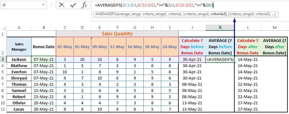
• Select average_range C3:I3 and press the F4 key thrice which will convert the range from the relative cell reference to the mixed cell reference (where the absolute column, but the relative row). So, the range is converted from C3:I3 ➪ $C3:$I3. As a result, if the formula copies downward, the column addresses (C to I) remain fixed, but the row numbers simultaneously changed (3, 4, 5, 6 …so on).   

• Similarly, select and convert criteria_range1 and criteria_range2 to the absolute cell reference (where both the column and the row numbers remain fixed) by pressing the F4 key once. So, the range is converted from C2:I2 ➪ $C$2:$I$2. As a result, if the formula copies downward, the column addresses (i.e., C to I) and the row number (i.e., 2) remain fixed (unchanged).

• Similarly, select and convert criteria1 and criteria2 to the mixed cell reference (where the absolute column, but the relative row) by pressing the F4 key thrice. So, the range is converted from J3 ➪ $J3 and B3 ➪ $B3. As a result, if the formula copies downward, the column addresses remain fixed, but the row numbers simultaneously changed.

=AVERAGEIFS($C3:$I3, $C$2:$I$2, “>=”&$J3, $C$2:$I$2, “<=”&$B3)

Press Enter to apply the formula. If the last parenthesis will close automatically if we do not close it.

Extending the Formula Till the End of the Range ➢ Alt+E+S+R / Alt+Ctrl+V+R

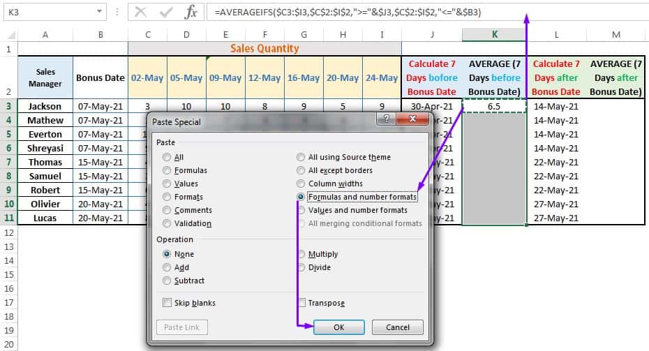
Copy the cell K3 with Excel shortcut Ctrl+C ➪ Making a selection of the entire ranges with Shift+ Right arrow (➡),  Down arrow (⬇) ➪ After copied the cell, press Alt+E+S+R ( sequentially press Alt, E, S, R) or press Alt+Ctrl+V+R (hold Alt+Ctrl+V, then press R) which will select the option ‘Formulas and number formats‘ in the ‘Paste Special’ dialog box ➪ Finally, click ‘OK’ or press ‘Enter’ from the keyboard to accept the formula.

■ To Calculate Average Sales 7 Days After The Bonus Date:

Similar to above, place an Excel AVERAGEIFS function in cell M3 to calculate average sales 7 days after the bonus date. 

=AVERAGEIFS($C3:$I3, $C$2:$I$2, “>=”&$B3, $C$2:$I$2, “<=”&$L3)

The difference from the above formula is the placement of criteria1 and criteria2. The date in cell L3 is greater than B3. Based on the concept, we place the criteria in the proper position in the formula. 

Secondly, proper application of cell references in the formula. 

Thirdly, the extension of the AVERAGEIFS formula till the end of the range without copying the cell format using ‘Formulas and number formats‘ in the Paste Special dialog box.

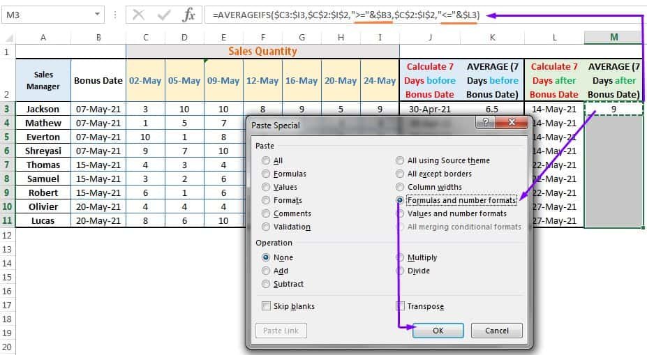
Press Enter to apply the formula. If the last parenthesis will close automatically if we do not close it.

(04) Using Special Character To Calculate Average by Using Excel AVERAGEIFS Function

■ To Use Asterisk Symbol:

An asterisk (*) symbol matches a series of zero or more characters. Please keep in mind that the asterisk symbol should be placed in the double quotation in the formula. For example, 

➢ s* – find a text string starting with the character ‘s’. For example, Shreyasi, Samuel, etc.

➢ *s – find a text string ending with the character ‘s’. For example, Thomas, Lucas, etc.

➢ *s* – find a text string containing the character ‘s’ (mentioned character may be present anywhere in the text string, for example, either at the starting, at the ending, or in between the text string, i.e., Jackson, Shreyasi).

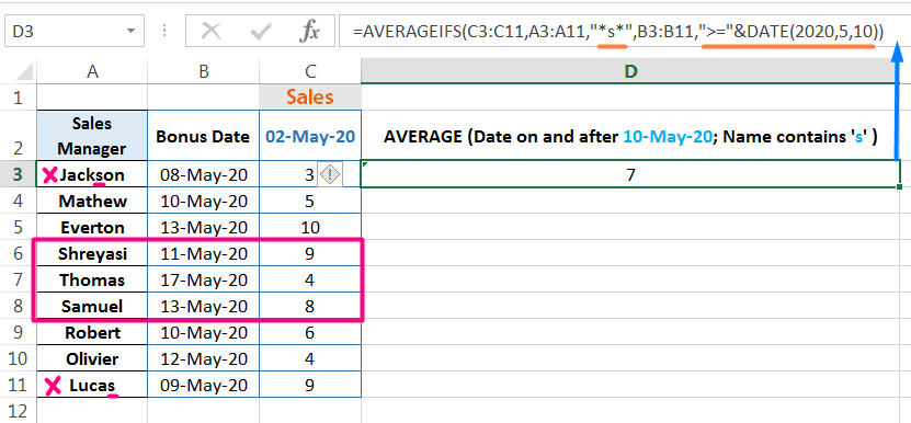
In the above example, we would like to calculate the average sales values based on two criteria: (01) the Sales Manager contains at least one character ‘s’ (02) Bonus Date should be greater than and equal to 10-May-2020.

=AVERAGEIFS(C3:C11, A3:A11, “*s*“, B3:B11, “>=”&DATE(2020,5,10))

The AVERAGEIFS function calculates the average of all sales values in the range C3:C11 if the corresponding cells in the range A3:A11 (Sales Manager) contain at least one character  ‘s’ or a series of characters ‘s’; and the corresponding cells in the range B3:B11 (Bonus Date) should be greater than or equal to 10-May-20.

The result returns 7 (average value). Total Sales of Shreyasi, Thomas, and Samuel is 9+4+8 =21. So average sales value is =21/3=7.

Note: The AVERAGEIFS formula ignoring the sales values of Jackson and Lucas, though they have characters ‘s’. In these cases, their bonus dates are less than 10-May-20.

■ To Use Question Mark Symbol:

A question mark (?) matches exactly one character. Similar to the asterisk symbol, a quotation mark should be placed in the double quotation in the formula. For example, 

➢ Lu”?“as – find a single character in exact position. For example, Lucas, Lumas, etc.

➢ “??????“ – find all the text strings containing six letters only. For example, Thomas, Samuel, Robert, etc.

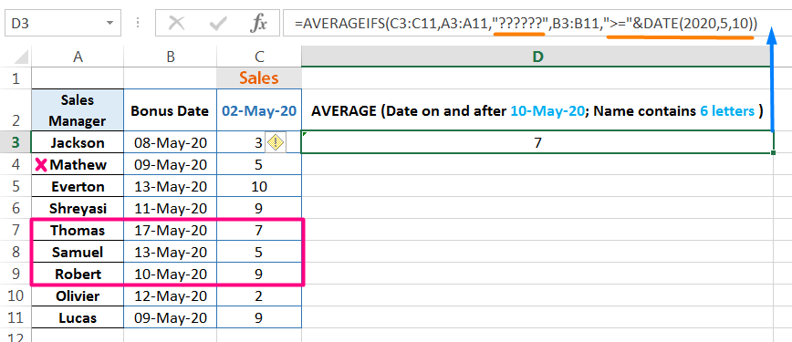
In the above example, we would like to calculate the average sales values based on two criteria: (01) Sales Manager with six letters (02) Bonus Date should be greater than and equal to 10-May-2020.

=AVERAGEIFS(C3:C11, A3:A11, “??????“, B3:B11, “>=”&DATE(2020,5,10))

The AVERAGEIFS function calculates the average of all sales values in the range C3:C11 if the corresponding cells in the range A3:A11 (Sales Manager) with six characters; and the corresponding cells in the range B3:B11 (Bonus Date) should be greater than or equal to 10-May-20.

The result returns 7 (average value). Total Sales of Thomas, Samuel, and Robert is 7+5+9 =21. So average sales value is =21/3=7.

Note: The AVERAGEIFS formula ignores the sales values of Mathew, though it has six letters. If we observe carefully, we found that the bonus date is less than 10-May-20.