The INDEX MATCH function Excel is often used together to make a nested formula that performs lookups. For example, both-way lookup or two-way lookup, reverse lookup, multiple criteria lookup, two-dimensional lookup, or 2-D lookup, case-sensitive lookup. 

The INDEX function is a lookup and reference function in Excel that returns a value at the intersection of a specified row and column. Whereas, the MATCH function is a lookup and reference function in Excel that searches through a range for a specific value and returns the relative position of a value within the range. 

The MATCH function is used to return the position of the item, not the actual item. Whereas the INDEX function not only retrieves the cell content or item, but it also moves to any row or column. Thus, the MATCH function is often used in conjunction with the INDEX function to make the INDEX MATCH formula that obtains an item in the same row of a table, but from a different column. 

While a single MATCH function is used within the INDEX function either as row_num or column_num and returns a value based on the single criterion (either row or column criterion), this type of lookup is called the one-dimensional lookup.  Similarly, while two MATCH functions are used within the INDEX function- one for the row_num and another for the column_num and returns a value based on the two criteria (both row and column criteria), this type of lookup in Excel is called the two-dimensional lookup or 2-D lookup. 

(I) The INDEX Function

In a cell, press the equality “=” sign to start the formula and just type a few letters ‘=ind….‘ and select the INDEX function from the given suggestion list with the help of a down arrow (↓), if required. 

Then press the ‘Tab’ key, INDEX syntax appears with the open parenthesis.

• The syntax for the INDEX Function

The INDEX function always returns a value or item specified by the intersection of the row_number and column_number. If the array contains only one row or column, the corresponding row_num or column_num argument is optional.

• Arguments of the INDEX Function

∴ Array or Reference is the one or several ranges, named range, or table;

∴ Row_num is the row number in the array (if omitted, column_num is required);

∴ Column_num is the column number in the array (if omitted, row_num is required);

∴ Area_num specifies which range from the reference argument to use. 

(01) If the array is one-dimensional that means it contains a single row or column, then both row_num and column_num are not required. 

For example, if we want to return the fourth item within a simple one-dimensional array using the following formula: 

=INDEX ({5,10,15,20,25,30}, 4)

Or, simply using the range =INDEX (A2:A6, 4)  

Which would return a value of 20, the fourth item in this array.

(02) The INDEX function is more frequently used with two-dimensional arrays or tables, where both  row_num and column_num are required. 

For example, =INDEX (A2:D6, 4, 2)

The INDEX function retrieves the item fourth rows down and two columns over a range. That means the formula would retrieve the item from the cell B4.

(03) If the array is two dimensional, which means it contains multiple columns and rows, and one of the arguments is omitted or set to zero, the INDEX function will return the whole row or column. 

For example, =SUM (INDEX (A2:D6 , , 2))

As a result, the entire B column is totaled.

(II) The MATCH Function

Similarly, press equality “=” sign in a cell to start the formula and just type a few letters “mat…” and select the MATCH function from the given suggestion list with the help of a down arrow (↓), if required.

Remember that upper and lower case doesn’t matter for typing the function, Excel by default converts it into the upper case. 

 Then press the ‘Tab’ key, by default MATCH syntax appears with an open parenthesis.

• The Syntax for the MATCH Function

• Arguments of MATCH Function

∴ Lookup_value is the item to match. It can be a number, text string, a logical value, or a reference.

∴ Lookup_array is the table or an array containing all of the values to search. 

∴ Match_type is a number that specifies how the match will be applied. 

• If match_type is zero (0), the MATCH function finds the first value/item in the array that is equal to lookup_value.

• If match_type is 1, the MATCH function finds the largest value less than or equal to lookup_value.

• If match_type is -1, the MATCH function finds the smallest value greater than or equal to lookup_value.

In the last two cases, the values in the lookup_array must be in ascending order for the MATCH function to work correctly. 

The match_type is optional and if we omit this argument, this argument is assumed to be 1.

(III) How Do INDEX MATCH Formula Performing in Excel? 

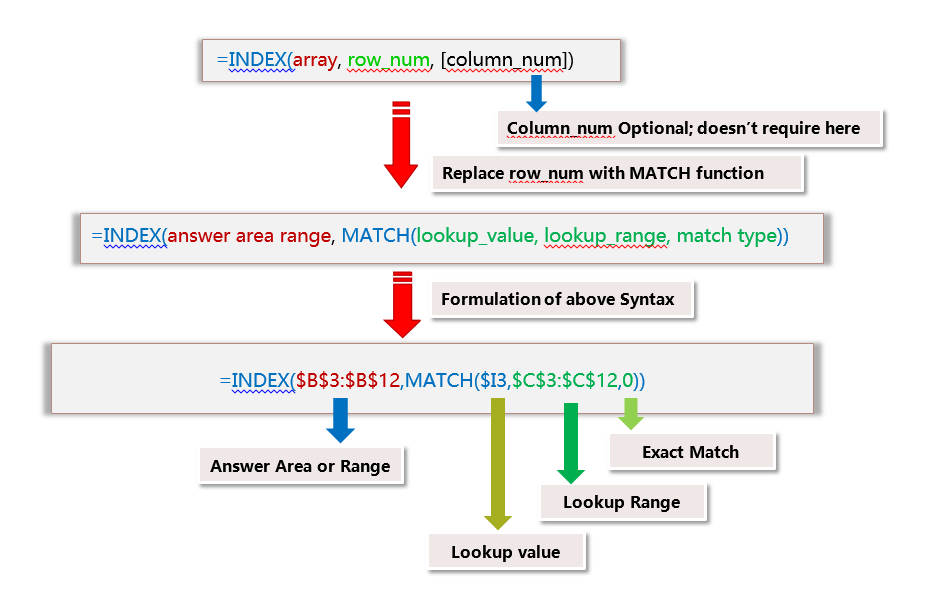
The INDEX-MATCH formula returns the value in a particular row and / or column of a given range of cells.  If the specified range of cells represents a single row, we need only specify a column reference (all of the cells are in the same row).

Similarly, If the specified range of cells represents a single column, we need only specify a row reference (all of the cells are in the same column). This single-way advance lookup is called the one-dimensional lookup.

If the specified range of cells contains both multiple rows and columns, in this case, the INDEX MATCH formula returns the value in the cell at the intersection of the specified row and column. This both-way advance lookup is called the two-dimensional lookup or the 2-D lookup.

A. INDEX MATCH Formula Performing the One-Dimensional LOOKUP:

• Syntax:

• Example:

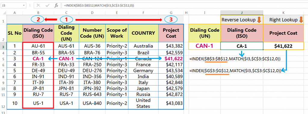
=INDEX($B$3 : $B$12, MATCH($I3, $C$3 : $C$12, 0))

We get the result for the ‘Dialing code (ISO)’ = CA-1

=INDEX($G$3 : $G$12, MATCH($I3, $C$3 : $C$12, 0))

We get the result for the ‘Project Cost’ = $41,622                                                            

If we observed both examples carefully, we find that only INDEX_array (answer area) changes in both cases. This is the key point for the INDEX MATCH formula with a one-dimensional lookup. 

B. INDEX MATCH Formula Performing the Two-Dimensional LOOKUP/ 2-D LOOKUP:

If we use two MATCH functions within the INDEX function – one for the row_num and another for the column_num, then the formula returns the value based on the matches between the row criteria and the column criteria. This type of lookup is called the two-dimensional lookup or the 2-D lookup.  

• Syntax:

• Example:

=INDEX($A$2 : $G$12, MATCH($I3, $C$2 : $C$12, 0), MATCH(J$2, $A$2 : $G$2, 0) )

We get the result for the ‘Dialing code (ISO)’ = CA-1

=INDEX($A$2 : $G$12, MATCH($I3, $C$2 : $C$12, 0), MATCH(K$2, $A$2 : $G$2, 0) )

We get the result for the ‘Project Cost’ = $41,622

If we observed both examples carefully, we find the two key points for the INDEX MATCH two-dimensional lookup:

(i) All the ranges selected as an INDEX_array, i.e., A2:G12

(ii) While the formula copied to another cell, only lookup_value within the second MATCH function (i.e., column lookup value) changes accordingly, e.g., J2, K2. 

(IV) What are the Merits of INDEX-MATCH Formula in Advanced Excel?

With the help of the INDEX MATCh formula, we can perform multiple activities based on multiple criteria:

• The INDEX MATCH function is performing Excel Reverse VLOOKUP | VLOOKUP to the left.

• The INDEX MATCH function is the best alternative of VLOOKUP Multiple Criteria in Excel.

• The INDEX MATCH function is the best alternative of Multiple VLOOKUP or Multiple columns VLOOKUP.

• INDEX, MATCH, and EXACT function altogether to perform a case-sensitive lookup.

(V) INDEX MATCH VS VLOOKUP – Which Function is Better in Excel?

➢ Don’t require to count the column number: Unlike the VLOOKUP function, we do not require to count the column numbers. Here we just select the answer column (for the INDEX MATCH formula) to get the result value.

➢ Safely inserting or deleting the columns: After inserting or deleting the columns in between the table_array, the VLOOKUP formula breaks — because the col_index_num within VLOOKUP couldn’t update automatically. Whereas the INDEX MATCH function independently works with the answer column, not with the count of columns, so it does not matter with the inserting or deleting of columns at all.

➢ Performing Reverse or Backward Lookup: The VLOOKUP function only performs to the right, whereas the INDEX MATCH formula performs a both-way lookup or two-way lookup, i.e., left and right of the lookup column. Left lookup is considered as reverse lookup or backward lookup. 

➢ Performing Two-Dimensional Lookup / 2-D Lookup: The INDEX MATCH MATCH formula or the VLOOKUP MATCH formula searches the match between the rows and columns criteria and returns the value. This feature in EXCEL is called the two-dimensional lookup / 2-D lookup.

➢ Performing with the multiple criteria: Another best feature of the INDEX MATCH formula is that the formula works with the multiple criteria, however, it is an array formula. To avoid array we can use the INDEX MATCH INDEX formula.

➢ Performing the Multiple Column Lookup / Multiple Lookup: Both the VLOOKUP formula and the INDEX MATCH formula are performing the multiple column lookup is called the Multiple Lookup.