5 years ago 3 years ago

06 ADVANCED USES OF EXCEL CHOOSE FUNCTION

by Sudipta Mondal 5 years ago3 years ago

4.9kviews

Excel CHOOSE function is very useful in advanced Excel because the CHOOSE formula returns the specific value from a list of values supplied as arguments.

Excel CHOOSE function is similar to the INDEX function in its simplest format. But, rather than an item being chosen from an array, the item is chosen from the list of arguments within the function.

TABLE OF CONTENTS:

(I). THE SYNTAX FOR THE EXCEL CHOOSE FUNCTION

Just type a few letters of the CHOOSE function, for example, ‘cho…‘ ➪ then select the Excel CHOOSE function from the given auto-suggested list with the help of a down arrow (↓), if required.

Then press the ‘Tab’ key which will select the CHOOSE function and the CHOOSE syntax appears with an open parenthesis.

(II). ARGUMENTS FOR THE EXCEL CHOOSE FUNCTION

➢ index_num – [required] the position of the value to return. It can be any number between 1 and 254, a cell reference (like A2, A3, etc.), or another formula (like RANDBETWEEN(3,7)).

➢ value1 – [required] the first value from which to choose.

➢ value2 – [optional] the second value from which to choose.

➢ value3 – [optional] the third value from which to choose….so on till 254.

value1, [value2], [value3],… : This can be the number (like 1,2,3,4,5), cell reference (like A2, B2, C2), ranges (A2:A10, B2:B10,C2:C10), text (‘January’, ‘February’,’ March’) or a formula.

The maximum number of values that can be provided is 254. The number of values provided should be ≥ index_value i.e., the value to choose. If the index_value is 3, then there should be at least three values: value1, value2, and value3. Otherwise, the formula returns an error #VALUE.

(III). EXAMPLES OF THE EXCEL CHOOSE FUNCTION

(01). EXCEL CHOOSE FUNCTION RETURNS A ‘VALUE’ BASED ON THE INDEX_NUM ARGUMENT

For a basic understanding of the Excel CHOOSE function, we explain with an example:

=CHOOSE(4,”Jan”,”Feb”,”Mar”,”Apr“,”May”,”Jun”,”Jul”,”Aug”,”Sep”,”Oct”,”Nov”,”Dec”)

CHOOSE formula will return Apr because the formula picked the value from the 4^th position based on the index_num, i.e., 4.

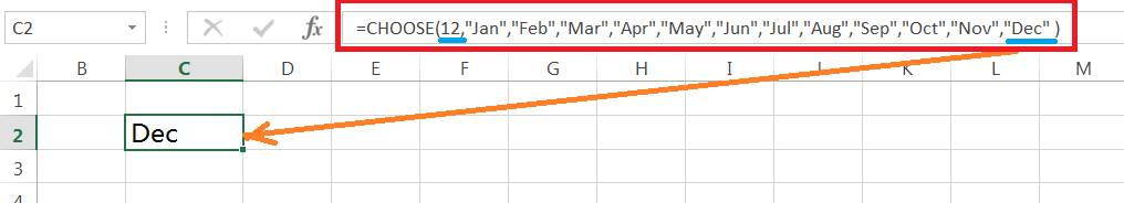
Similarly, =CHOOSE(12,”Jan”,”Feb”,”Mar”,”Apr”,”May”,”Jun”,”Jul”,”Aug”,”Sep”,”Oct”,”Nov”,”Dec“)

CHOOSE formula will return Dec because the formula picked the value from the 12^th position based on the index_num, i.e., 12.

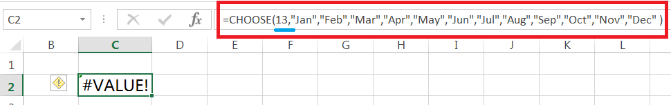
CHOOSE function returns a value based on the index_num argument-3

If the index_number is greater than the provided values, the function will give an error #VALUE!

In the above example, we have taken 12 months list. So the index_number must be in between the value of 1 to 12. If we put index_number more than that, such as 13, then the Excel CHOOSE function will return an error #VALUE!.

CHOOSE function returns a value based on the index_num argument-2

(02). EXCEL CHOOSE FUNCTION RETURNS A CUSTOM DAY / MONTH FROM A DATE

If we want to get a weekday name and a month name from a date, we must use the Excel CHOOSE function in the following way:

To get a Weekday name from a Date in cell C3

=CHOOSE(WEEKDAY(B3),”Sun”,”Mon”,”Tue”,”Wed”,”Thu”,”Fri”,”Sat”)

To get a Month name from a Date in cell D3

=CHOOSE(MONTH(B3),”Jan”,”Feb”,”Mar”,”Apr”,”May”,”Jun”,”Jul”,”Aug”,”Sep”,”Oct”,”Nov”,”Dec”)

Finally, press Enter to accept the formula. Formula ends by default and closes the last parenthesis if not placed.

➢ COPY THE ‘FORMULAS’ TILL THE END OF THE RANGE

After applying the CHOOSE formula in cells C3 and D3, copy the formula till the end of the range by the Excel shortcut Alt+E+S+R (sequentially press Alt, E, S, R) or Alt+Ctrl+V+R (press Alt+Ctrl+V, then R) which will select the ‘Formulas and number formats‘ in the “Paste Special” dialog box ➪ then press Enter or click OK.

➢ CONVERT ALL THE ‘FORMULAS’ INTO ‘VALUES

It is very good practice to convert all the unnecessary formulas into values, otherwise, the Excel file becomes heavy in size and sometimes formulas return an error due to the deletion of the source file.

We can convert all the formulas into values either in two ways:

➢ Using the ‘Values and number formats‘ option in the ‘Paste Special’ dialog box by the Excel shortcut Alt+E+S+U (sequentially press Alt, E, S, U) / Alt+Ctrl+V+U (press Alt+Ctrl+V, E, S, then U) ➪ press Enter or click on OK.

➢ Alternatively, Using the ‘Values‘ option in the ‘Paste Special’ dialog box by the Excel shortcut Alt+E+S+V (sequentially press Alt, E, S, V) / Alt+Ctrl+V+V (press Alt+Ctrl+V, E, S, then V) ➪ press Enter or click on OK.

(03). EXCEL CHOOSE FUNCTION RETURNS A ‘VALUE’ BASED ON CONDITIONS || BEST ALTERNATIVE OF NESTED IF FUNCTION

We generally used the nested IFs function to get the values based on suggested multiple conditions, but the Excel CHOOSE function is the best alternative method to get the result.

For example, if we want to label the result based on the marks obtained by students, we should follow the formula:

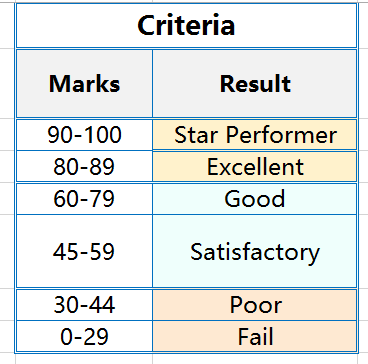
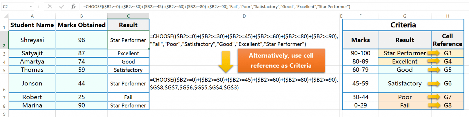
CHOOSE function returns a value based on Conditions-1

CHOOSE function returns a value based on Conditions-2

Based on the obtained marks in cell B2, we label the criteria in cell C2 with the CHOOSE formula as follows:

=CHOOSE(($B2>=0) + ($B2>=30) + ($B2>=45) + ($B2>=60) + ($B2>=80) +($B2>=90), “Fail”, “Poor”, “Satisfactory”, “Good”, “Excellent”, “Star Performer”)

Note:

➢ Always arrange the conditions in the CHOOSE function in ascending order (i.e., the criteria value starts from lowest to highest). In the above example, the lowest value starts from 0 (consider the Marks between 0-29) and the highest value of 90 (consider the Marks between 90-100).

➢ Instead of manually typing the criteria, we can use the cell reference as criteria and will get the same result. As a result, the formula becomes more dynamic.

=CHOOSE(($B2>=0)+($B2>=30)+($B2>=45)+($B2>=60)+($B2>=80)+($B2>=90), $G$8, $G$7, $G$6, $G$5, $G$4, $G$3)

• $G$8 – use absolute cell reference and refers to the cell containing ‘Fail’.

• $G$7 – use absolute cell reference and refers to the cell containing ‘Poor’.

• $G$6 – use absolute cell reference and refers to the cell containing ‘Satisfactory’.

• $G$5 – use absolute cell reference and refers to the cell containing ‘Good’.

• $G$4 – use absolute cell reference and refers to the cell containing ‘Excellent’.

• $G$3 – use absolute cell reference and refers to the cell containing ‘Star Performer’.

➢ If we want to copy the formula to another cell, always try to fix the cell reference using the dollar sign ($) by pressing the F4 key.

➢ After putting all the arguments in the CHOOSE formula, press Enter to accept the formula. Formula ends by default and closes the last parenthesis if not placed.

➢ COPY THE ‘FORMULAS’ TILL THE END OF THE RANGE

➢ CONVERT ALL THE ‘FORMULAS’ INTO ‘VALUES

It is very good practice to convert all the unnecessary formulas into values, otherwise, the Excel file becomes heavy in size and sometimes formulas return errors due to the deletion of the source file.

We can convert all the formulas into values either in two ways:

Note: If we do not arrange the conditions in the CHOOSE function or arrange in descending order (i.e., the criteria value starts from highest to lowest) then the CHOOSE formula does not work properly and gives the wrong/inappropriate/incorrect output. The below example is given for reference:

(04). EXCEL CHOOSE FUNCTION IS USED FOR ‘CALCULATION’ BASED ON CONDITIONS || BEST ALTERNATIVE OF NESTED IF FUNCTION

We can use the Excel CHOOSE function to calculate the dataset based on multiple conditions and the CHOOSE formula is considered as the best alternative to the Nested IFs function.

As in the given example, we can calculate the commission of each sales manager based on their sales.

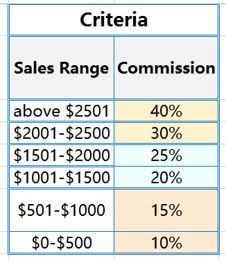
Excel CHOOSE function is used for Calculations based on Conditions-1

Based on the Sales Amount in cell B2, we calculate the commission in cell C2 with the CHOOSE formula as follows:

=CHOOSE(($B2>=0) + ($B2>=501) + ($B2>=1001) + ($B2>=1501) + ($B2>=2001) +($B2>=2501), $B2*10%, $B2*15%, $B2*20%, $B2*25%, $B2*30%, $B2*40%)

➢ Always arrange the conditions in the CHOOSE function in ascending order (i.e., the criteria value starts from lowest to highest). In the above example, the lowest value starts from 0 (consider the Sales Range between $0-$500) and the highest value from 2501 (consider the Sales Range above $2501).

➢ The CHOOSE formula becomes more dynamic if we can use the cell reference as criteria and will get the same result easily.

=CHOOSE(($B2>=0)+($B2>=501)+($B2>=1001)+($B2>=1501)+($B2>=2001)+($B2>=2501), $B2*$G$8, $B2*$G$7, $B2*$G$6, $B2*$G$5, $B2*$G$4, $B2*$G$3)

• $G$8 – use absolute cell reference and refers to the cell containing commission criteria 10%.

• $G$7 – use absolute cell reference and refers to the cell containing commission criteria 15%.

• $G$6 – use absolute cell reference and refers to the cell containing commission criteria 20%.

• $G$5 – use absolute cell reference and refers to the cell containing commission criteria 25%.

• $G$4 – use absolute cell reference and refers to the cell containing commission criteria 30%.

• $G$3 – use absolute cell reference and refers to the cell containing commission criteria 40%.

➢ If we want to copy the formula to another cell, always try to fix the cell reference using the dollar sign ($) by pressing the F4 key.

➢ After putting all the arguments, press Enter to accept the formula. Formula ends by default and closes the last parenthesis if not placed.

➢ COPY THE ‘FORMULAS’ TILL THE END OF THE RANGE

➢ CONVERT ALL THE ‘FORMULAS’ INTO ‘VALUES

We can convert all the formulas into values either in two ways:

Note: We never arrange the conditions in the CHOOSE function in descending order (i.e., the criteria value starts from highest to lowest), otherwise the CHOOSE formula does not work properly and gives the wrong/inappropriate/incorrect output.

(05). EXCEL VLOOKUP & CHOOSE FUNCTION COMBINEDLY USED FOR ‘VLOOKUP MULTIPLE CRITERIA’

Both the VLOOKUP and CHOOSE functions combined to form a nested formula that performs Excel VLOOKUP multiple criteria.

• Excel VLOOKUP & CHOOSE function with Helper column makes a non-array formula

• Excel VLOOKUP & CHOOSE function without Helper column makes an array formula

➢ A. VLOOKUP MULTIPLE CRITERIA: VLOOKUP & CHOOSE FUNCTIONS WITH HELPER COLUMN (NON-ARRAY FORMULA)

In the case of Excel VLOOKUP multiple criteria, if we use the VLOOKUP CHOOSE nested formula along with a Helper column will make a non-array formula.

SYNTAX:

STEPS TO START:

• Step 1: Insert a Helper column before the table_array (that is the starting of the dataset) and it is mandatory to create a single criterion for using the VLOOKUP function.

• Step 2: Then apply the CONCATENATE() function in the first cell of the helper column (i.e., the cell A3) to make a unique criterion. We can apply any of the below 02 methods for concatenation.

➢ Either use the ampersand (&) symbol for concatenation, for example =C3 & “*” & D3

➢ Or, use the CONCATENATE() function, for example =CONCATENATE(C3, “*”, D3)

Copy the formula till the end of the range. Please note that we use an asterisk symbol “*” as the separator for concatenating. Because in some cases, two different criteria give the same result after combination. Instead of the asterisk, we may use hyphen “-“, underscore “_”, slash “/” as a separator.

• Step 3: Select the cell where to start the VLOOKUP formula and get the result of VLOOKUP Multiple Criteria (i.e., the cell J3).

After selecting the cell, place an equality “=” sign to start the formula and just type a few letters of VLOOKUP such as “=vlo…“ and select the VLOOKUP function from the Excel auto-suggested function list with the help of a down arrow (↓), if required.

Promptly press the ‘Tab’ key which will select the VLLOKUP function and the VLOOKUP syntax appears with an open parenthesis.

• Step 4: Select the lookup_value, the first argument of the VLOOKUP function.

Select the multiple criteria from multiple cells or multiple columns, for example from the cells H3 and I3, and simultaneously, concatenate them with an ampersand (&) symbol. Moreover, we use a separator in the double quotations between the criteria, for example, the asterisk symbol “*”.

Then we fix the cell reference for getting the dynamic result. Select the lookup_value argument with the cursor and fix only the column addresses by pressing three times the F4 key. Thus the range is converted from the relative to the mixed cell reference where it indicates the absolute column and the relative row.

As a result, while the formula is copied to the right side or horizontally, the column address does not change but the row address changes accordingly.

=VLOOKUP ($H3 & “*” & $I3,

Place a comma (,) which indicates the completion of the current argument and pass a command to move to the next argument i.e., table_array.

• Step 5: In place of the table_array, the second argument of the VLOOKUP function, we will apply the CHOOSE function.

The CHOOSE() function returns the specific value from a list of values supplied as arguments.

Just type a few letters of the CHOOSE function, for example, ‘cho…‘ and select the CHOOSE function from the given auto-suggested list with the help of a down arrow (↓), if required.

Remember that upper and lower case doesn’t matter for typing the function, Excel by default converts it into the upper case.

Then press the ‘Tab’ key and as a result, the CHOOSE syntax appears with the open parenthesis. We need to fill up all the required arguments in the CHOOSE function.

After applying the CHOOSE formula it looks like this:

=VLOOKUP ($H3 & “*” & $I3, CHOOSE({1,2}, $A$2:$A$20, $F$2:$F$20)

➢ Inside the CHOOSE function, we can put the integer values in the curly brackets {} separated with comma (,) that will refer to a range of cells or columns likes CHOOSE({1,2}.

Remember that according to the requirement, we can put 3, 4, 5… so on till 254.

➢ Index number 1 always refers to the lookup column, after that any index number (2, 3, 4… so on) can refer to any column in our database either to the right side or to the left side of the lookup column.

➢ Index number 1 always refers to the lookup column range (i.e., here is the Helper column) A2 : A20. It is mandatory otherwise formula doesn’t work at all. Select the range and makes it absolute from relative cell reference by pressing the F4 key once and the range looks like $A$2 : $A$20. As a result, the range does not change when the formula is copied to another cell either horizontally or vertically.

➢ Index number 2 refers to the column range having answers (is called answer_range answer_range) i.e., F2 : F20. Similarly, select the range and makes it absolute from relative cell reference by pressing the F4 key once, and the range looks like $F$2 : $F$20.

• Step 6: After closing the parenthesis of the CHOOSE function, place a comma (,) which indicates the completion of the current argument and pass a command to move to the next argument i.e., col_index_ num, the third argument of the VLOOKUP function.

Be careful that our answer value is present in the second column range (is called answer_range i.e., F2:F20) which is referred to by 2. So we put the value 2 in place of column_index_num.

=VLOOKUP ($H3 & “*” & $I3, CHOOSE({1,2}, $A$2:$A$20, $F$2:$F$20), 2

• Step 7: Place a comma (,) and move to the last argument of the VLOOKUP function is range_lookup. In this case, we are looking for an exact match, thus put the value zero (0) or FALSE.

=VLOOKUP ($H3 & “*” & $I3, CHOOSE({1,2}, $A$2:$A$20, $F$2:$F$20), 2, 0

• Step 8: Finally, press Enter to accept the formula. Formula ends by default and closes the last parenthesis as well. Copy the formula till the end of the range. The complete formula looks like this:

=VLOOKUP ($H3 & “*” & $I3, CHOOSE({1,2}, $A$2:$A$20, $F$2:$F$20), 2, 0)

The formula returns the result 7,510 in cell J3 as a Sales ($) value.

• Step 9: CONVERT ALL THE ‘FORMULAS’ INTO ‘VALUES’

We can convert all the formulas into values either in two ways:

➢ Using the ‘Values and number formats’ option in the ‘Paste Special’ dialog box by the Excel shortcut Alt+E+S+U (sequentially press Alt, E, S, U) / Alt+Ctrl+V+U (press Alt+Ctrl+V, E, S, then U) ➪ press Enter or click on OK.

➢ Alternatively, Using the ‘Values’ option in the ‘Paste Special’ dialog box by the Excel shortcut Alt+E+S+V (sequentially press Alt, E, S, V) / Alt+Ctrl+V+V (press Alt+Ctrl+V, E, S, then V) ➪ press Enter or click on OK.

➢ B. VLOOKUP MULTIPLE CRITERIA: VLOOKUP & CHOOSE FUNCTIONS WITHOUT HELPER COLUMN (ARRAY FORMULA)

In the case of Excel VLOOKUP multiple criteria, if we use the VLOOKUP CHOOSE nested formula without a Helper column will make a non-array formula.

SYNTAX:

STEPS TO START:

• Step 1: Select the cell where to start the VLOOKUP formula and get the result of VLOOKUP Multiple Criteria (i.e., the cell I3).

Promptly press the ‘Tab’ key which will select the VLOOKUP function and the VLOOKUP syntax appears with an open parenthesis.

• Step 2: Select the lookup_value, the first argument of the VLOOKUP function.

Select the multiple criteria from multiple cells or multiple columns, for example from the cells G3 and H3, and simultaneously, concatenate them with an ampersand (&) symbol. Moreover, we use a separator in the double quotations between the criteria, for example, the asterisk symbol “*”.

As a result, while the formula is copied to the right side or horizontally, the column address does not change but the row address changes accordingly.

=VLOOKUP ($G3 & “*” & $H3,

Place a comma (,) which indicates the completion of the current argument and pass a command to move to the next argument i.e., table_array.

• Step 3: In place of the table_array, the second argument of the VLOOKUP function, we will apply the CHOOSE function.

The CHOOSE() function returns the specific value from a list of values supplied as arguments.

Just type a few letters of the CHOOSE function, for example, ‘cho…‘ and select the CHOOSE function from the given auto-suggested list with the help of a down arrow (↓), if required.

Remember that upper and lower case doesn’t matter for typing the function, Excel by default converts it into the upper case.

Then press the ‘Tab’ key and as a result, the CHOOSE syntax appears with the open parenthesis. We need to fill up all the required arguments in the CHOOSE function.

After applying the CHOOSE formula it looks like this:

=VLOOKUP ($G3 & “*” & $H3, CHOOSE({1,2}, $B$2:$B$20 & “*” & $C$2:$C$20, $E$2:$E$20),

➢ In the CHOOSE function, we can put the integer values in the curly brackets {} separated with comma (,) that will refer to a range of cells or columns likes CHOOSE({1,2}.

As per our requirement, we can put 3, 4, 5… so on till 254.

Index number 1 always refers to the lookup column range. We make two criteria ranges into a single lookup range. For example, there are two ranges B2:B20 and C2:C20, and make them into a single range by concatenating with an ampersand sign (&). In between them, we use an asterisk symbol “*” as a separator, like B2:B20 & “*” & C2:C20.

It is a mandatory step otherwise formula doesn’t work at all. Select the range and makes it absolute from relative cell reference by pressing once F4 key, like $B$2:$B$20 & “*” & $C$2:$C$20. As a result, the range does not change when the formula is copied to another cell either horizontally or vertically.

➢ Index number 2 refers to the column range having answers (answer_range) i.e., E2: E20. Similarly, select the range and makes it absolute from relative cell reference by pressing the F4 key once, such as $E$2: $E$20.

• Step 4: After closing the parenthesis of the CHOOSE function, place a comma (,) which indicates the completion of the current argument and pass a command to move to the next argument i.e., col_index_ num, the third argument of the VLOOKUP function.

Our answer value is present in the second column range (is called answer_range i.e., E2:E20) which is referred to by 2. So we put the value 2 in place of column_index_num.

=VLOOKUP ($G3 & “*” & $H3, CHOOSE({1,2}, $B$2:$B$20 & “*” & $C$2:$C$20, $E$2:$E$20), 2,

Place a comma (,) which indicates the completion of the current argument and pass a command to move to the next argument i.e., range_lookup.

• Step 5: The last argument of VLOOKUP is range_lookup. As we are looking for an exact match, thus we consider the last argument as zero (0) or FALSE.

=VLOOKUP ($G3 & “*” & $H3, CHOOSE({1,2}, $B$2:$B$20 & “*” & $C$2:$C$20, $E$2:$E$20), 2, 0

• Step 6: Since this is an array formula, press Ctrl+Shift+Enter to accept the formula, instead of just Enter. By default curly brackets {} placed before and after the formula.

Then the complete formula looks like this:

{=VLOOKUP ($G3 & “*” & $H3, CHOOSE({1,2}, $B$2:$B$20 & “*” & $C$2:$C$20, $E$2:$E$20), 2, 0)}

Only the copy-paste an array formula into the other cells, Excel does not allow at all. In this case, we drag the cell with the formula end of the range with the fill handle, it is a small square in the bottom-right corner of the selected cell.

As a result, we get the result in Total Sales ($) for the first instance is 7,510.

• Step 7: CONVERT ALL THE ‘FORMULAS’ INTO ‘VALUES’

Always try to convert all the formulas in the dataset into values in any of the following two ways:

(06). EXCEL VLOOKUP & CHOOSE FUNCTION COMBINEDLY USED FOR ‘REVERSE VLOOKUP’

Excel Reverse VLOOKUP – is used to VLOOKUP to the left and is a useful formula in data analysis and big data handling.

The VLOOKUP function searches value only to the right, but the VLOOKUP and CHOOSE function can perform in both directions from the lookup column – VLOOKUP to the left and VLOOKUP to the right. This feature of Excel VLOOKUP is called both-way lookup or two-way lookup.

The VLOOKUP and CHOOSE nested formula is more flexible than VLOOKUP and retrieves values from the left of the lookup column is called the Reverse VLOOKUP or VLOOKUP backwards, which means a reverse lookup is a part of the both-way lookup.

The Excel CHOOSE function returns the specific value from a list of values supplied as arguments. We use this feature of the CHOOSE function in the VLOOKUP function as a table_array to perform the Excel Reverse VLOOKUP.

The VLOOKUP and CHOOSE nested formula performs VLOOKUP to the left that means the formula retrieves the value from the left of the lookup_column.

➢ SYNTAX:

➢ STEPS TO START:

Steps of Excel REVERSE VLOOKUP: with VLOOKUP & CHOOSE function (One-Dimensional Lookup)

• Step 1: Select the cell where to start the VLOOKUP formula and get the result of the Reverse VLOOKUP (i.e., the cell J3).

Promptly press the ‘Tab’ key which will select the VLOOKUP function and the VLOOKUP syntax appears with an open parenthesis.

• Step 2: Select the lookup_value, the first argument of the VLOOKUP function, locates in cell I3, and fix the Column address by pressing the F4 key three times. It looks like $I3. So the cell is converted from the relative to the mixed cell reference where it indicates the absolute column and relative row.

As a result, while the formula is copied to the right side or horizontally, the column addresses do not change at all but the row addresses change accordingly.

=VLOOKUP($I3,

Place a comma (,) which indicates the completion of the current argument and pass a command to move to the next argument i.e., table_array.

• Step 3: In place of the table_array, the second argument of the VLOOKUP function, we will apply the CHOOSE function.

The CHOOSE() function returns the specific value from a list of values supplied as arguments.

Just type a few letters of the CHOOSE function, for example, ‘cho…‘ and select the CHOOSE function from the given auto-suggested list with the help of a down arrow (↓), if required.

Remember that upper and lower case doesn’t matter for typing the function, Excel by default converts it into the upper case.

Then press the ‘Tab’ key which will select the CHOOSE function and the CHOOSE syntax appears with the open parenthesis. We need to fill up all the required arguments in the CHOOSE function.

After applying the CHOOSE formula it looks like this:

=VLOOKUP($I3, CHOOSE({1,2,3} , $C$3 : $C$12, $B$3 : $B$12 ,$G$3 : $G$12),

➢ In the CHOOSE function, we can put the integer values in the curly brackets {} separated with comma (,) that will refer to a range of cells or columns likes CHOOSE({1,2,3}.

As per our requirement, we can put 4, 5, 6… so on till 254.

➢ Index number 1 always refers to the lookup column range i.e., C3:C12. It is mandatory otherwise formula doesn’t work at all. Select the range and makes it absolute from the relative cell reference by pressing the F4 key once. The range looks like $C$3:$C$12. As a result, the range does not change when the formula is copied to another cell either horizontally or vertically.

➢ Index number 2 refers to the column range is placed on the left side of the lookup value i.e., B3:B12. Similarly, select the range and makes it absolute from the relative cell reference by pressing the F4 key once. The range looks like $B$3:$B$12. As a result, the range does not change when the formula is copied to another cell either horizontally or vertically.

Remember that, it is optional and we can refer to the column range on the right side of the lookup value column instead of the left.

➢ Index number 3 refers to the column range is placed on the right side of the lookup value i.e., G3:G12. Similarly, select the range and makes it absolute from the relative cell reference by pressing the F4 key once. The range looks like $G$3:$G$12. As a result, the range does not change when the formula is copied to another cell either horizontally or vertically.

Remember that, it is optional and we can refer to the column range on the left side of the lookup value column instead of the right.

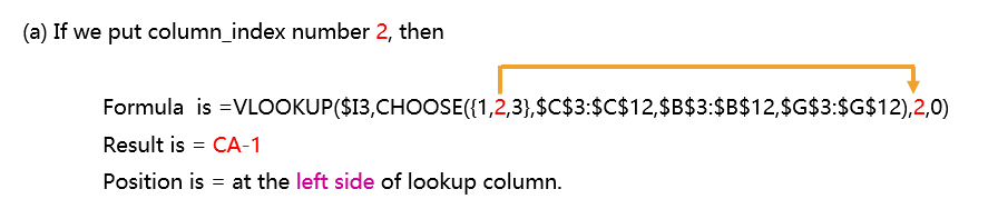
• Step 4: After closing the parenthesis of the CHOOSE function, place a comma (,) which indicates the completion of the current argument and pass a command to move to the next argument i.e., col_index_ num, the third argument of the VLOOKUP function.

➢ Performing Reverse VLOOKUP / VLOOKUP to the LEFT/ VLOOKUP Backwards

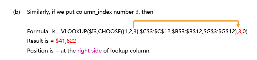
➢ Performing RIGHT VLOOKUP / VLOOKUP to the RIGHT

The VLOOKUP and CHOOSE function combinedly form a nested formula that can retrieve the value from both on the left and right sides of the lookup column. This phenomenon is called the both-way lookup or two-way lookup.

Place a comma (,) which indicates the completion of the current argument and pass a command to move to the next argument i.e., range_lookup.

• Step 5: The last argument of VLOOKUP is range_lookup. As we are looking for an exact match, thus we consider the last argument as zero (0) or FALSE.

• Step 6: Finally, press Enter to accept the formula. Formula ends by default and closes the last parenthesis as well. Copy the formula till the end of the range. The complete formula looks like this:

=VLOOKUP($I3, CHOOSE({1,2,3} , $C$3 : $C$12, $B$3 : $B$12 ,$G$3 : $G$12), 2, 0)

➪ The formula returns the result: CA-1

=VLOOKUP($I3, CHOOSE({1,2,3} , $C$3 : $C$12, $B$3 : $B$12 ,$G$3 : $G$12), 3, 0)

➪ The formula returns the result: $41,622

• Step 7: Convert All the ‘Formulas’ into ‘Values’

We can convert all the formulas into values either in two ways:

(IV). CONCLUSION

• The index_value can vary between 1 to 254.

• The number of values can also vary from 1 to 254.

• VALUE! Error – Occurs when:

➢ The number of values should be equal or more than the index_num but if it is less than index_num will return a #VALUE error, that means always index_num ≥ values.

➢ If the index_num is less than 1, the formula returns an error #VALUE!

➢ The given index_num argument is non-numeric.

• #NAME? Error – This occurs when the value arguments are text values that are not enclosed in quotes and are not valid cell references.

• Values can be the cell reference (A2, B2, C2), or the ranges (A2:A10, B2:B10, C2:C10, etc), text (‘January’, ‘February’,’ March’ etc.), or a formula.

• The CHOOSE formula returns different values based on conditions, but inside the formula, conditions should be arranged in ascending order.

• Excel CHOOSE function will not retrieve the value from a range or array constant (such as A2:C10).

If you would like to improve your academic and professional career as well, then the below courses help you a lot. Instead of Advanced Excel, a number of best courses suggested you through this platform that boosts your confidence and flies your career high.