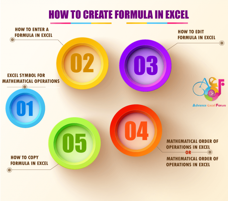
How To Create Formula in Excel? But before we go into details we must have knowledge of the formula, functions, mathematical operations, order of precedence or mathematical order of operations, cell reference and use of the dollar sign in excel, etc.
The Formulas are the basic component of Excel. They link together and manipulate the data in the worksheet. Formulas can be used to perform basic arithmetic, carry out more complex if-then-else analysis, or search through lists of data to look up and match specific criteria. In addition to allowing us to create our own formulas, Excel comes with hundreds of built-in-formulas called functions, which are used to perform frequent calculations, such as SUM, AVERAGE, COUNT, COUNTA, or more complex calculations, such as Double VLOOKUP, Nested VLOOKUP or NPV (net present value).
A formula is an expression that calculates numbers or evaluates the contents of one or more cells. A function is a predefined formula in Excel that is made available for us to use in Excel, such as SUM, VLOOKUP, SUMIFS, etc.
A formula combines specific values, cell references (or cell addresses), mathematical operations, and/or functions used in a calculation. When a cell reference (or cell address) is included in a formula, it is not the address that is used in the formula but, rather, the value that is in that cell. The result of the expression is placed in the cell that contains the formula, but the formula is displayed in the formula bar.
All formulas consist of:
➢ An underlying formula that is entered into the cell;
➢ A resulting value is displayed in the cell.
In this tutorial, we will learn how to use mathematical operations (operators) in Excel formulas, the mathematical order of operations, and learn how to construct formulas using cell addresses so that when the value of an input cell changes, the result of the formula dynamically changes without modification in the formula.
TABLE OF CONTENTS:
Toggle01. EXCEL SYMBOL FOR MATHEMATICAL OPERATIONS
An operator is a symbol that determines the type of operation we want the formula to perform. In other words, Excel operators signify the type of computation that takes place between the cells and the linked values.
Most of the basic Excel formulas require nothing but the sole use of operators. Excel recognizes four types of operators: such as Arithmetic, Reference, Comparison, and Single text.
➢ Arithmetic Operator: They are by far the most common type of operator and they combine numbers, cell addresses, and functions to perform calculations. Most of these operators are straightforward, but the exponentiation operator might require further explanation. The formula =a^b means that the value a is raised to the power b. For example, the formula =5^5 produces 3125 (that is, 5*5*5*5*5=3125).
➢ Reference Operator: The reference operators combine two cell references or ranges to create a single joint reference.
➢ Comparison Operator: A comparison operator compares two or more numbers, text strings, cell contents, or function results. If the statement is true, the result of the formula is given the logical value TRUE, which is equivalent to any nonzero value. If the statement is false, the formula returns the logical value FALSE, which is equivalent to zero. This type of operator mostly used in Excel’s logical functions.
➢ Single Text Operator: A text operator in a formula that returns text. Text operator uses the ampersand (&) symbol to work with text cells, text strings enclosed in quotation marks, and text function results.
Table: Excel’s Mathematical Operation based on Excel Operators
| Type | Operator | Description | Function | Example | Result |
| Arithmetic Operator | + | Plus Sign | Addition | =5+5 | 10 |
| – | Minus Sign | Subtraction | =5-5 | 0 | |
| * | Asterisk | Multiplication | =5*5 | 25 | |
| / | Forward Slash | Division | =5/5 | 1 | |
| ^ | Exponent symbol | Exponentiation | =5^5 | (5*5*5*5*5*) =3125 | |
| % | Percentage | Percentage (Divides the value by 100) | =20% | 0.2 | |
| Reference Operator |
, | Comma |
Union operator. Combines multiple cells or range references into one reference |
=SUM(A1,B1:B10,D1:E10) |
Returns summation value from the mentioned cells or range of cells. |
| : | Colon |
Range operator. Defines the selected range. |
=SUM(B1:B10) | Returns summation value from the mentioned range of cells. | |
| Space |
Intersection operator. Produces one reference to cells common to two references |
=SUM(B1:B10 B1:D10) |
Returns summation value from the mentioned cells common to two references. | ||
| Reference Operator |
> | Greater than |
|
=A1>B1 |
If the value of cell A1 is greater than cell B1 returns ‘TRUE’ otherwise ‘FALSE’. |
| < | Less than |
|
=A1<B1 |
If the value of cell A1 is less than cell B1 returns ‘TRUE’ otherwise ‘FALSE’. | |
| = | Equals to |
Equates the values and |
=A1=B1 |
If the value of cell A1 is equal to cell B1 returns ‘TRUE’ otherwise returns ‘FALSE’. | |
| >= | Greater than or equal to |
|
=A1>=B1 |
If the value of cell A1 is greater than or equal to cell B1 returns ‘TRUE’ otherwise returns ‘FALSE’. | |
| <= | Less than or equal to |
|
=A1<=B1 |
If the value of cell A1 is less than or equal to cell B1 returns ‘TRUE’ otherwise returns ‘FALSE’. | |
| <> |
Angle Brackets |
Not equal to |
=A1<>B1 |
If the value of cell A1 is not equal to cell B1 returns ‘TRUE’ otherwise returns ‘FALSE’. | |
|
Single Text Operator |
& |
Ampersand |
Connects different entries |
=B1&”/”&C1 |
02. HOW TO ENTER A FORMULA IN EXCEL?
Formulas can be entered in one of 05 ways, described below. However, Excel has 03 different input modes that determine how Excel interprets certain keystrokes and mouse actions.
(i) When we type the equal sign to begin the formula, Excel goes into Enter mode, which is the mode we use to enter text such as the formula’s operands and operators.
(ii) If we press any keyboard navigation key such as Page Up, Page Down, or any arrow key, or if we click any other cell in the worksheet or click on any worksheet, Excel enters Point mode. This is the mode we use to select a cell or range as a formula operand. When we are in Point mode, we can use any of the standard range-selection techniques. Note that Excel returns to Enter mode as soon as we type an operator or any character.
(iii)If we press the F2 key, Excel enters Edit mode, which is the mode we use to make changes to the formula. For example, when we are in Edit mode, we can use the left and right arrow keys or Home and End keys and move the cursor to another part of the formula for deleting or inserting characters. Moreover, we can also enter Edit mode by clicking anywhere within the formula. Finally, press F2 to return to Enter mode.
Note: Notice that on the left side of the status bar, Excel denotes which mode is currently in: Enter, Point, or Edit.
• METHOD 1: TYPING FORMULA MANUALLY INTO A CELL

1. Click the cell in which we want to enter a formula.
2. Type equality sign (=) or plus sign (+). Excel displays the formula in the Formula bar and in the active cell.
3. Type the formula’s operands and operators.
4. Press Enter or Ctrl+Enter to confirm the formula.
• METHOD 2: CREATING THE FORMULA USING THE CELL REFERENCE

1. Click the cell in which we want to enter a formula.
2. Type equality sign (=) or plus sign (+) to begin the formula. Excel displays the formula in the Formula bar and in the active cell.
3. Click the first cell we want to reference in the formula. Excel inserts the cell reference into the formula. Remember that we do not include any spaces in the formula.
4. Type an Excel operator for the formula requirement. For example, if we want to SUM then use the ‘+’ plus sign. Similarly, if we want to tally the values between two cells then use ‘=” equal to sign etc.
5. Click the next cell we want to reference in the formula. Excel inserts the cell reference into the formula.
4. Press Enter to accept the formula. The formula results appear in the cell. To view the formula, simply click the cell. The Formula bar displays any formula assigned to the active cell.
■ Note: If we change any of the values in the cells referenced in the formula, the formula results automatically update to reflect the changes.
➢ Equal Sign Mandatory: If you type A1+B1 without the equal sign, Excel does not recognize that you entered a formula and stores the “formula” as text.
➢ Ignore Upper- or Lowercase: When we create a formula, type the cell references either in uppercase, such as =B2+B3, or lowercase, such as =b2+b3, Excel changes cell references to uppercase automatically.
➢ Using Cell Reference in Excel: It is the best practice to use cell references instead of actual values in formulas because these references enable our formulas to work dynamically with the data contained in those cells or ranges. Additionally, when we drag or copy our formula horizontally or vertically to other cells, cell references have been changed. In this case, we can use 03 types of references according to the requirement.
■ Relative Cell Reference: The row and column references can change when we copy the formula to another cell because the references are actually offset from the current row and column. By default, Excel creates relative cell references in formulas. (for example, A1).
■ Absolute Cell Reference: The row and column references don’t change when we copy the formula because the reference is to an actual cell address. An absolute reference uses two dollar signs in its address: one for the column letter and one for the row number (for example, $A$1).
■ Mixed Cell Reference: Either the row or the column reference is relative, and the other is absolute.
⇒ Row Absolute: The reference is partially absolute. When we copy the formula, the column part adjusts, but the row part does not change. For example, A$1
⇒ Column Absolute: The reference is partially absolute. When we copy the formula, the row part adjusts, but the column part does not change. For example, $A1
■ Note: We had detail explained on Cell Reference in a separate tutorial. Request you read this tutorial: 03 Types of Excel Cell Reference: Relative, Absolute & Mixed
HOW TO USE A DOLLAR SIGN IN EXCEL?
(01) We can convert a general number format into a currency format attached with a dollar sign.
(02) In the formula, a Dollar sign ($) is often used to fix the cell reference. An Excel Cell Reference is a cell address that identifies a cell’s location in the worksheet, based on its column letter and row number.
We can quickly switch a cell reference from relative to absolute or mixed. Rather than retyping the formula in every new cell, select the cell reference or range and then repeatedly press the F4 key, Excel cycles through the different reference types – starting with the relative reference, followed by the absolute reference, then to a mixed reference with an absolute row address, followed by a mixed reference with an absolute column address.
Excel cell reference switches in this order: C2:F12 ➪ $C$2:$F$12 ➪ C$2:F$12 ➪ $C2:$F12

However, we can manually insert the dollar symbols ($) in Excel in the appropriate positions of the cell address.
• METHOD 3: INSERTING FUNCTIONS INTO FORMULAS USING THE ‘FORMULA AUTOCOMPLETE TOOL’
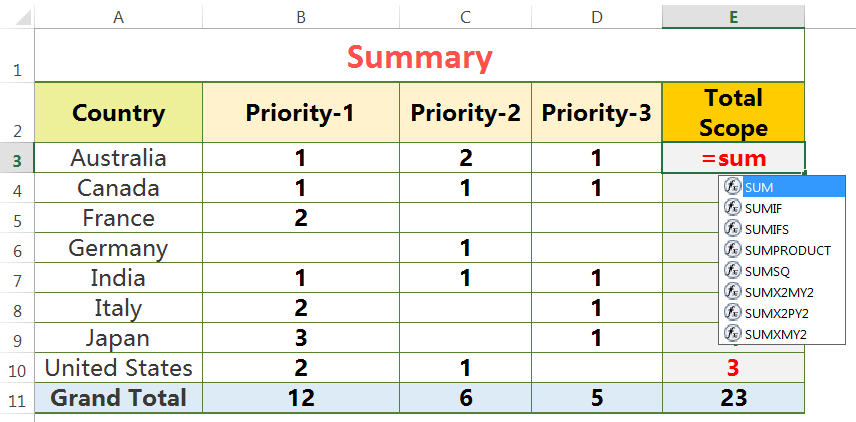
(01) Select the cell where to apply the function. Here, we apply the SUM function for adding the values ➪ place equality sign (=) and type sum, Excel by default select the SUM function from the drop-down list; otherwise select the SUM function with down navigation arrow (⬇).
Note that the upper or lower case does not matter for syntax, Excel by default considers it in upper case.
(02) Then press the Tab key which allows us to open the SUM function with an open parenthesis.
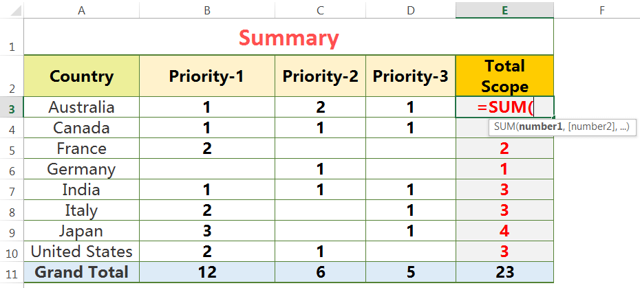
(03) Select the range.
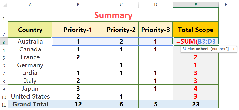
(04) Then press Ctrl+Enter or Enter to accept the formula.
• METHOD 4: INSERTING FUNCTIONS INTO FORMULAS USING THE ‘INSERT FUNCTION’ DIALOG BOX
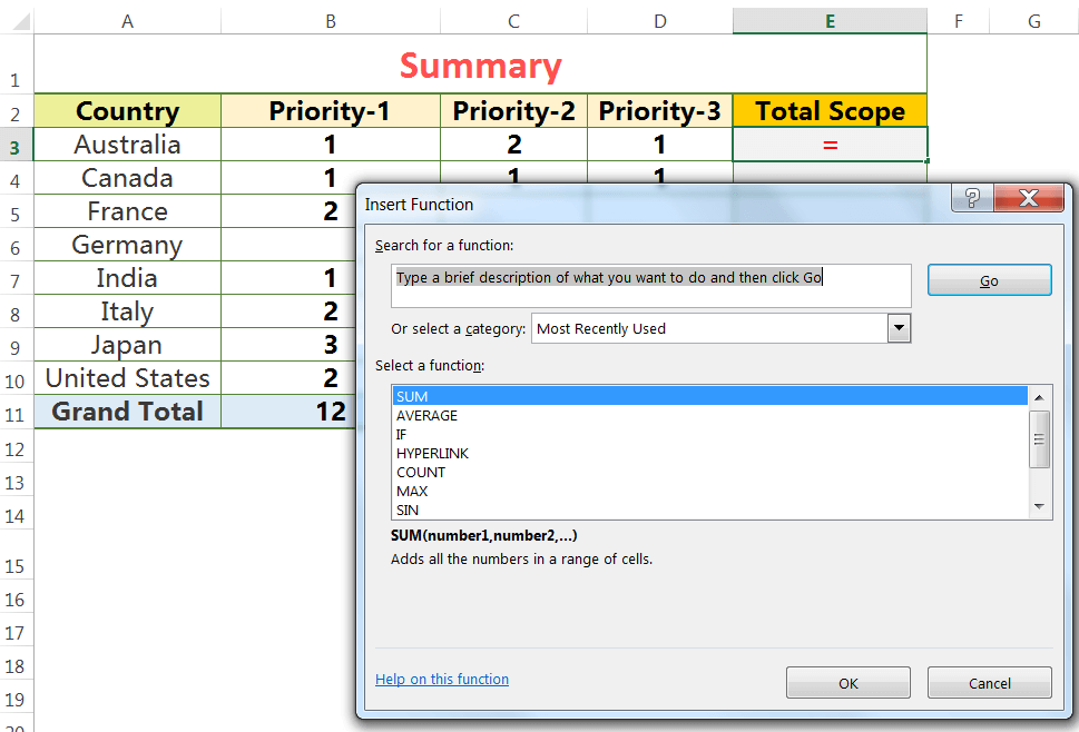
(01) Select the cell where to apply the function in the formula. Here, we apply the SUM function for adding the values.
(02) Press Shift+F3 which will open the ‘Insert Function’ dialog box. Excel automatically place an equal sign (=) in the cell.
➢ Type and Search SUM function in ‘Search for a function:’ box ➪ then click OK or,
➢ Click to choose a category from ‘Or select a category:’ drop-down list, for example, select ‘Math & Trig’ category and find the SUM function using the horizontal scroll bar ➪ then click OK.
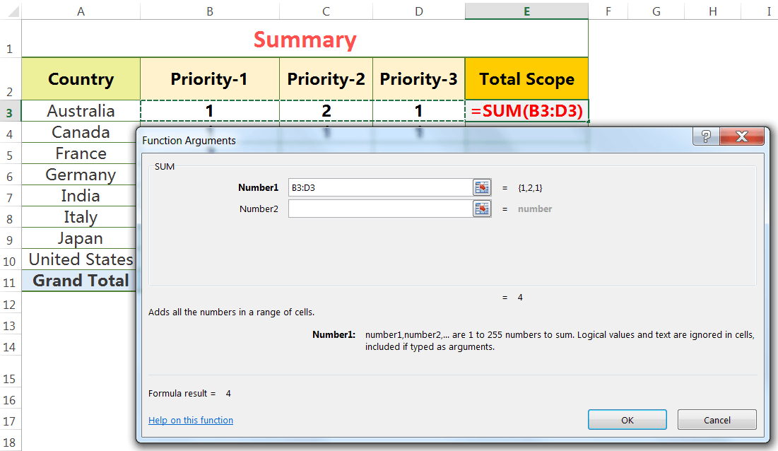
(03) As a result, another ‘Function Arguments’ dialog box opens ➪ selects the range (i.e., B3:D3) in the Number1 box; similarly we can select multiple different ranges ➪ Press Enter or click OK to accept the formula.
• METHOD 5: INSERTING FUNCTIONS INTO FORMULAS USING THE ‘INSERT FUNCTION’ BUTTON ON THE FORMULA BAR
(01) Select the cell where to apply the function, such as in this case we apply SUM function for adding the values.
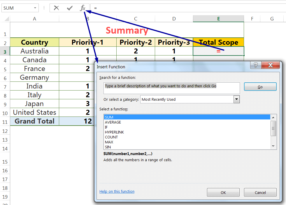
(02) Click the ‘Insert Function’ button (fx) on the formula bar which will open the ‘Insert Function’ dialog box. Excel automatically place an equal sign (=) in the cell.
Either type and search SUM function in the ‘Search for a function:’ box or click to choose a category from ‘Or select a category:’ drop-down list and select the SUM function ➪ then click OK.
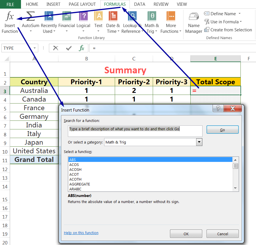
Alternatively, go to the ‘Formulas’ tab ➪ click the ‘Insert Function’ button (fx) in the function library group.
(03) As a result, another ‘Function Arguments’ dialog box opens ➪ selects the range (i.e., B3:D3) in the Number1 box; similarly we can select multiple different ranges ➪ Press Enter or click OK to accept the formula.
One of the most popular functions available in Excel is the AutoSum function. AutoSum automatically totals the contents of cells.
Excel AutoSum is a formula that calculates (by default) the total from the adjacent cell up to the first non-numeric cell using the SUM() function in its formula. The AutoSum feature provides a quick way to sum a contiguous range of numbers (that means there are no empty cells in a range). The range may be a single cell or thousands of cells.
We can apply the AutoSum function in 03 ways:
➢ METHOD 1: APPLY AUTOSUM IN EXCEL BY KEYBOARD SHORTCUT (ALT+=)
(01) Click a cell beneath a contiguous range or a cell right to the contiguous range where we want to insert a sum total.
(02) Press Alt + = which will apply AutoSum and Excel by default select the suggested range (or drag to select the desired range).
(03) Finally, press Enter to accept the formula.
■ Note: We had detail explained on Excel Shortcuts in two separate tutorials. Request you read these tutorials:
80+ Excel Shortcuts with ALT Key || Best Hotkey of Keyboard Shortcuts
90+ Best Excel CTRL Shortcuts | Useful Keyboard Shortcuts |
➢ METHOD 2: APPLY AUTOSUM IN EXCEL BY CLICKING THE AUTOSUM ICON IN THE ‘HOME’ TAB
(01) Click a cell beneath a contiguous range or a cell right to the contiguous range where we want to insert a sum total.
(02) Go to the Home tab ➪ click Autosum Icon in the Editing group. As a result, Excel by default selects the suggested range (or drag to select the desired range).
(03) Press the Enter key to accept the formula.
➢ METHOD 3: APPLY AUTOSUM IN EXCEL BY CLICKING AUTOSUM ICON IN THE ‘FORMULAS’ TAB
(01) Click a cell beneath a contiguous range or a cell right to the contiguous range where we want to insert a sum total.
(02) Go to the Formulas tab ➪ click Autosum Icon in the Function Library group. Similarly, Excel by default selects the suggested range (or drag to select the desired range).
(03) Press the Enter key to accept the formula.
■ Note: We had detail explained on Excel Autosum in a separate tutorial. Request you read this tutorial: 03 Useful Methods : Add Numbers With AutoSum Excel
03. HOW TO EDIT FORMULA IN EXCEL?
If we make changes to our worksheet, we may need to edit formulas. Excel gives us 03 ways to enter Edit mode and make changes to a formula in the selected cell.
(01) Before editing a cell, first click the cell that we want to edit.
(02) Apply any of the 03 methods for formula editing
➢ Press F2.
➢ Double-click the cell.
➢ Select the formula cell that we want to edit and then click in the Formula bar.
(03) Use the arrow keys to navigate to the character we want to change.
(04) Using the Backspace key, delete any unwanted characters left to the cursor and use the Delete key for the deletion of any unwanted characters right to the cursor.
and type any additional characters.
(05) After making any changes in the formula, press the Enter key to accept the formula.
■ Note:
• If the cell contains a formula that returns an error, Excel will display a small triangle in the upper-left corner of the cell. Activate the cell, and we’ll see a Smart Tag. If we click the Smart Tag and choose one of the options for correcting the error. (The options will vary according to the type of error in the cell.)
• During editing a formula, we can select multiple characters either by dragging the mouse cursor over them or by pressing Shift and the navigation keys.
• If we just remove the initial equal sign (=), the formula converted to text, and if we type the initial equal sign to convert the cell contents back to a formula.
04. MATHEMATICAL ORDER OF OPERATIONS IN EXCEL
Or, ORDER OF PRECEDENCE IN EXCEL
Excel evaluates a formula according to a predefined order of precedence. The order of operations (also called the order of precedence) are the rules that control the sequence in which arithmetic operations are performed, which affects the result of the calculation. Excel always performs mathematical calculations left to right in the below order:
Table: The Excel Order of Precedence
| Operator | Operation | Order of Precedence |
| ( ) | Parenthesis | 1st |
| : | Range | 2nd |
| <space> | Intersection |
3rd |
| , | Union |
4th |
| – | Negation | 5th |
| % | Percentage |
6th |
| ^ | Exponentiation |
7th |
| / and * | Division and Multiplication | 8th |
| + and – | Addition and Subtraction |
9th |
| & | Concatenation |
10th |
| = < > <= >= <> |
Comparison |
11th |
■ Note:
(01) USING OF SAME ORDER PRECEDENCE IN FORMULAS
Note the multiplication and division have the same order precedence as well as the comparison operators. If the formula contains operators with the same order precedence then Excel will evaluate the operators from left to right. For example,
consider the formula =24*12/3.
∴ Excel will evaluate the multiplication operator first because it is left positioned. As a result, the answer we get is 96 (24*12 equals 288, and 288/3 equals 96).
∴ If we perform the division first, the answer we get is 96 ( 12/3 equals 4, and 24*4 equals 96). So, we can say on the basis of the arithmetic rule, Excel prioritizes the division operator instead of the multiplication operator.
Similarly, consider the formula =24/12*3
∴ In this case, Excel will evaluate the division operator first because it is left positioned. As a result, the answer we get is 6 ( 24/12 equals 2, and 2*3 equals 6).
(02) USING OF PARENTHESES IN FORMULAS
Parentheses in formulas confirm that a lower-order operation occurs first. For example, consider the formula =(24+12)/3 where addition within the parentheses occurs first instead of the division since division has a higher order of operations than addition. The answer from the calculation we get is 12 ( 24+12 equals 36, and 36/3 equals 12).
05. HOW TO COPY FORMULA IN EXCEL?
A. COPY FORMULAS WITH AUTOFILL

We can use Excel’s AutoFill feature to quickly copy formulas across rows or columns in the worksheets. If the cell references in a formula are relative, Excel automatically adjusts the formula for the destination cell.
(01) Click the cell containing the formula we want to copy.
(02) Point to the fill handle in the bottom-right corner of the cell until the pointer changes to the fill pointer (a thin black plus sign) across or down the number of cells to which we want to copy the formula.

(03) Drag or double click the fill handle to copy the formula. As a result, Excel copies the formula into each cell. Cell references in copied formulas adjust based on their relative locations to the original formula.
■ Note: In the case of absolute cell referencing, Excel keeps the absolute cell reference the same regardless of where we copy the formula. Remember that Absolute cell references include two dollar signs in the formula, preceding the column letter and row number.
Please keep in mind that by this method, the same cell formatting (color, font, border, etc) copied to the new range of cells.

B. COPY FORMULAS WITH EXCEL SHORTCUT (CTRL+C)
(01) Click the cell containing the formula and copy it by pressing the Excel shortcut Ctrl+C (alternatively, Home ➪ Clipboard ➪ Copy).
(02) Extend the selection end to the cell or range of cells where to copy the formula by pressing the Shift and Navigation arrow keys and then press Ctrl+V or press Enter to accept the formula (alternatively, Home ➪ Clipboard ➪ Paste).

If the formula’s cell references are relative, Excel adjusts the formula for the new cell to which we move the formula. If the formula’s cell references are absolute, Excel keeps the cell references the same regardless of the new location in the worksheet.
■ Note: Similarly, by this method, the same cell formatting (color, font, border, etc) copied to the new range of cells.

C. COPY FORMULAS VERTICALLY WITH THE EXCEL SHORTCUT (CTRL+D)
(01) Click the cell containing the formula.
(02) Select the new cell or range of cells vertically / column-wise by pressing the Shift and Down navigation arrow key (⬇) considering the first cell having a formula.

(03) Then press Ctrl+D.
As a result, the formula copied to the cell ranges vertically (or, column-wise).
■ Note: Similarly, by this method, the same cell formatting (color, font, border, etc) copied to the new range of cells.

D. COPY FORMULAS HORIZONTALLY WITH THE EXCEL SHORTCUT (CTRL+R)
(01) Click the cell containing the formula.
(02) Then select the new cell or range of cells horizontally / row-wise by pressing the Shift and Right navigation arrow key (➡) considering the first cell having a formula.
(03) Then press Ctrl+R.

As a result, the formula copied to the cell ranges horizontally (or, row-wise).
■ Note: Similarly, by this method, the same cell formatting (color, font, border, etc) copied to the new range of cells.

E. COPY FORMULAS WITH THE ‘PASTE SPECIAL’ DIALOG BOX
When pasting data, Paste Special is the best option because it has several options for inserting values, formulas, formatting, or links to the original source data into the new location. Additionally, using the paste special method, we can easily avoid copied cell formatting to the new range of cells. Paste options are available in 03 ways:
➢ by the Excel shortcut;
➢ from the Paste menu in the clipboard group (Home ➪ Clipboard ➪ Paste ➪ Paste Special command); and
➢ from the Paste Options menu on the mouse right-click.
Step to Start:
(01) Select and copy (Ctrl+C) the cell containing the formula.
(02) Extend the selection end to the cell or range of cells where to copy the formula by pressing the Shift and Navigation arrow keys. We can include the copied cell having a formula in the selection.
(03) Then use Excel Shortcut Alt+E+S+R (sequentially press Alt, E, S, R) or Alt+Ctrl+V+R (press Alt+Ctrl+V, R) which will select the ‘Formulas and number formats’ option in the Paste Special dialog box.

(04) Then press Enter or click OK.
As a result, the formula is copied to the cell ranges.
■ Note: By this method, no cell formatting (color, font, border, etc) copied to the new range of cells.

06. HOW TO EXACT COPY FORMULA IN EXCEL?
When we paste a formula to a different location, Excel adjusts the formula’s cell references based on a new location. Sometimes, for a single cell or small dataset, we can make an exact copy of the formula by converting the cell references to absolute references — but this isn’t always desirable.
A. EXACT COPY THE FORMULA FROM THE FORMULA BAR (APPLICABLE ONLY FOR SINGLE CELL)

1. Select cell E3.
2. Select and copy the formula from the formula bar.
Alternatively, press the F2 key to activate edit mode and then press Ctrl+Shift+Home to move the cursor to the start of the formula and select all the formula text. Or we can drag the mouse to select the entire formula.
Note that use Ctrl+Shit+End to select the entire formula when the formula is more than one line long, but optional for formulas that are a single line.
3. Press Ctrl+C (or Choose Home ➪ Clipboard ➪Copy).
This copies the selected formula to the Clipboard.
4. Press Esc to end edit mode
5. Select cell F3 and press F2, for edit mode.
7. Press Ctrl+V (or Choose Home ➪ Clipboard ➪ Paste), followed by Enter.
This operation pastes an exact copy of the formula text into cell F3.

■ Note: By this method, we can paste the formula only in one cell instead of multiple cells. If we try to paste the formula in multiple cells, Excel returns us a warning message

B. EXACT COPY THE FORMULA WITH TEXT TO COLUMNS (APPLICABLE ONLY FOR SINGLE COLUMN)
Another advanced method to copy the exact formula to the range of cells arranged in a single column by the Text to Columns because of text to columns only applicable for a single column. If we want to copy formulas from multiple columns then we apply similar steps repeatedly for every column. With the help of Text to Columns, We can convert the formulated cells in a column to ‘text’ and paste them easily to a new location.
Step to Start:
(i) Either select only the range (i.e., E2:E11) or select the entire column (i.e. column E). Here we select the entire column by pressing Ctrl+Spacebar. Remember that no merge cells exist there.
(ii) Then press Alt+D+E (sequentially press Alt, D, E) or Alt+A+E (sequentially press Alt, A, E) which will open the ‘Convert Text to Columns Wizard‘.
➢ In Step 1 of 3, by default Delimited is selected ➪ Press Enter or click Next.

➢ In Step 2 of 3, by default, all the checkboxes remain unchecked, except Tab checkbox ➪ Press Enter or click Next.

➢ In Step 3 of 3, by default, the ‘General’ option is selected but we select the ‘Text’ option radio button ➪ Then press Enter or click Finish.

As a result, all the cells with the formula converted to text, and the formula in the cell is exposed.

(iii) Copy the range of cells (i.e., E2:E11) with a keyboard shortcut Ctrl+C and paste them in the desired location (i.e., in cell B14 and pasted range is B14:B23).
As a result, the text range remains the same (unmodified) in the pasted area.

(iv) In the next step, again we convert the range from ‘Text’ to ‘General’ with the help of ‘Convert Text to Columns Wizard’.
Press Alt+D+E (sequentially press Alt, D, E) or Alt+A+E (sequentially press Alt, A, E) which will open the ‘Convert Text to Columns Wizard‘.
➢ In Step 1 of 3, by default Delimited is selected ➪ Press Enter or click Next.

➢ In Step 2 of 3, by default, all the checkboxes remain unchecked, except Tab checkbox ➪ Press Enter or click Next.

➢ In Step 3 of 3, by default, the ‘General’ option is selected but we select the ‘Text’ option radio button ➪ Then press Enter or click Finish.

As a result, the text is converted to general and the formula is exactly copied to the new location.

■ Note: We had detail explained on Convert Text to Columns Wizard in a separate tutorial. Request you read this tutorial: 10 Examples of Text to Columns || How to Split Cells/Columns in Excel
C. EXACT COPY THE FORMULA WITH ‘PASTE SPECIAL‘ (APPLICABLE FOR ENTIRE RANGES)
We can exactly copy the entire range along with the formula using the ‘Paste Special’ dialog box and easily paste it to another location.
➢ METHOD 1: At first, Select the entire range by Ctrl+A and then copy it by Ctrl+C ➪ Then select only the first cell where to paste the range ➪ Press Alt+E+S+R (sequentially press Alt, E, S, R) or Alt+Ctrl+V+R (press Alt+Ctrl+V, then R) which will select the ‘Formulas and number formats‘ in the Paste Special dialog box ➪ Finally press Enter or click OK to accept the formula.
■ Note: We can also avail the ‘Formulas’ option in the Paste Special dialog box using the Excel shortcut Alt+E+S+F (sequentially press Alt, E, S, F) or Alt+Ctrl+V+F (press Alt+Ctrl+V, then F)

As a result, the range with formula is pasted over a new location without copying any formatting.

➢METHOD 2: If we want to copy both formula and cell formatting from the copied range then follow the following steps:
(i) CHANGE THE COLUMN WIDTH: At first, Select the entire range by Ctrl+A and then copy it by Ctrl+C ➪ Then select only the first cell where to paste the range ➪ Press Alt+E+S+W (sequentially press Alt, E, S, W) or Alt+Ctrl+V+W (press Alt+Ctrl+V, then W) which will select the ‘Column widths‘ in the Paste Special dialog box ➪ Finally press Enter or click OK to accept the formula.
As a result, similar column widths from the copied range has been adjusted to the new location.

(ii) PASTE THE FORMULAS AND NUMBER FORMATS: Simultaneously, press Alt+E+S+R (sequentially press Alt, E, S, R) or Alt+Ctrl+V+R (press Alt+Ctrl+V, then R) which will select the ‘Formulas and number formats‘ in the Paste Special dialog box ➪ Finally press Enter or click OK to accept the formula.
As a result, the formulas and the number formats from the copied range are copied to the new location.

(iii) PASTE THE FORMATTING: Simultaneously, press Alt+E+S+T (sequentially press Alt, E, S, T) or Alt+Ctrl+V+T (press Alt+Ctrl+V, then T) which will select the ‘Formats‘ option in the Paste Special dialog box ➪ Finally press Enter or click OK to accept the formula.

As a result, similar formatting from the copied range is pasted to the new location.

■ Note: We had detail explained on Excel Paste Special in a separate tutorial. Request you read this tutorial: Paste Special in Excel Vs Break Link – Which one is Better?
D. EXACT COPY THE FORMULA WITH ‘FIND AND REPLACE’ (APPLICABLE FOR ENTIRE RANGES)
We can replace the equality sign with uncommon text, then paste the range to another location and finally replace this uncommon text with an equality sign.
(i) Select the range with Ctrl+A ➪ then press Ctrl+H which will open the ‘Find and Replace‘ dialog box.
➢ type equality (=) sign in front of the ‘Find what:’ box.
➢ type any uncommon text such as ‘change’ in front of the ‘Replace with:’ box.

At last, press the Replace All button, and Excel replaces all the equality signs with the text ‘change’ in the entire range.

(ii) Select the entire range with Ctrl+A ➪ then copy with shortcut Ctrl+C ➪ paste it to another location ➪ then press Ctrl+H which will open the ‘Find and Replace‘ dialog box.
➢ type the text ‘change’ in front of the ‘Find what:’ box.
➢ type equality (=) sign in front of the ‘Replace with:’ box.

Finally, press the Replace All button, and Excel replaces all the text ‘change’ with equality (=) signs in the entire range. As a result, the formula restored in a new location and works perfectly.

■ Note: We had detail explained on Find and Replace in a separate tutorial. Request you read this tutorial: 07 Points Guided You How to Find And Replace in Excel?

Premium Courses on ed2go
Premium Courses on Coursera
Premium Courses on Udemy

12 Examples || How to Use Excel Go To Special?
07 Points Guided You How to Find And Replace in Excel?
05 Points Should Learn How to Freeze Panes in Excel?
12 Things Guided You How to Manage An Excel Workbook
03 Useful Methods : Add Numbers With AutoSum Excel
04 Simple to Advanced Methods: How to Filter in Excel?
05 Best Ways: Create Password Protect Excel & Unprotect it
08 Best Examples: How to Use Excel Conditional Formatting?
04 BEST WAYS: HOW TO TRANSPOSE DATA IN EXCEL
Tutorial 01: How to Use Excel SUMIFS Function with Single & Multiple Criteria
Thanks for your interest joining to Advance Excel Forum community.
Something went wrong.

Join Our Community List
Subscribe to our mailing list and get interesting stuff and updates to your email inbox.
* VERIFY & CONFIRM YOUR EMAIL * We respect your privacy and take protecting it seriously*.


